The development of a background paper and the application of cost effectiveness indicators for use in Section 32 requests under Ontario Regulation 419: air pollution – local air quality
This report recommends a methodology for evaluating the cost effectiveness and relative effectiveness of potential air contaminant reduction techniques. It’s intended to support decisions regarding the appropriateness of potential air contaminant reduction techniques for industrial operations.
Cost Effectiveness Methodology
1.1 Introduction
This report recommends a methodology for evaluating the cost effectiveness of potential air contaminant reduction techniques as well as an indicator of relative effectiveness. The cost effectiveness methodology and indicator are intended to support decisions regarding the appropriateness of potential air contaminant reduction techniques for industrial operations.
Evaluation of air contaminant reduction techniques is based upon technical feasibility and effectiveness. However, the decision to implement is based upon efficiency and appropriateness. Efficiency is generally a measure of resources used (i.e. equipment, utilities, personnel, etc.). A contaminant reduction technique that is effective at reducing an air contaminant and uses resources effectively may be appropriate to implement.
Alternatively, a contaminant reduction technique that is effective at reducing an air contaminant, but uses resources inefficiently may be inappropriate to implement. The common measure of resources is cost. All resources can be converted into units of cost. Consequently, assessment of cost effectiveness of a potentially feasible technique would be valuable for informing a decision regarding appropriateness. Further, an indicator value that points to a threshold level at which cost effectiveness may be appropriate would provide an additional metric for a decision.
Importantly, cost effectiveness is a measure of efficiency in achieving an objective and not an evaluation of the benefit of achieving the objective. A cost effectiveness evaluation is not a cost benefit analysis. The recommended methodology presents a measure of the total resource effectiveness of a potentially feasible air contaminant reduction technique to be used as a tool in deciding the appropriateness to implement.
1.2 Background
Air management in Ontario changed significantly in November, 2005 with enactment of Ontario Regulation 419: Air Pollution – Local Air Quality (Regulation 419) and amendments in August, 2007. Regulation 419 establishes new or updated air standards based upon a scientific assessment of the health and environmental effects of contaminants. In the past, air quality standards were developed through a combination of scientific, technical and economic considerations. Under Regulation 419, technical and economic issues are now considered separately in the alteration of standards process set out in section 32.
A request for approval of an alteration to a standard for a contaminant in Schedule 3 of Regulation 419 may be made if circumstances listed in section 32 are applicable. A Schedule 3 air standard may be replaced with a site-specific standard that accounts for technical considerations and, if requested, economic feasibility. A request for approval of an alteration to an air standard must include the supporting information specified in section 32 of the regulation. Among other things, the request should include a technical benchmarking report for the identification and selection of methods that are best suited to minimizing Point of Impingement (POI) concentrations of the relevant contaminant. The request must demonstrate to the director of the Ministry of the Environment (designated under section 32, Regulation 419), that “best efforts” are being used to comply with the standard(s) set out in Schedule 3 of Regulation 419 and/or that POI concentrations are being reduced as much as possible. The Ministry’s Standards Development Branch (SDB) is responsible for development and implementation of the process to assess the acceptability of a request for approval of an alteration to a standard and may approve such requests pursuant to section 32(21) of Regulation 419.
1.2.1 Technology Benchmarking Reports
A technology benchmarking report is required to be submitted as part of a request for an alteration to a standard. Development of a technology benchmarking report and the identification of best practices is a regulatory requirement as set out in paragraphs 3 through 6 of subsection 32(13) of Regulation 419. Technology benchmarking is a key component of the Ministry’s risk-based approach to addressing situations where eligible facilities are requesting approval of an alteration to a standard. The purpose of a technology benchmarking report is to ensure that the actions taken represents best practices in limiting the POI concentrations and impacts of a contaminant(s).
Identification of available techniques and technology including an assessment of feasibility given site-specific considerations is required in a technology benchmarking report. The report should demonstrate a relatively thorough evaluation of available options to reduce POI concentrations of contaminant(s) for which an alteration to a standard is being requested. For significant sources of contaminant(s) a thorough review of POI reduction techniques should include an evaluation of the following:
- Materials: The assessment should consider a comprehensive review of the various potential raw material(s) used and how they affect emissions of contaminants of concern. Specific attention should be provided in identifying availability and feasibility of material changes that could reduce POI concentrations.
- Processes: The assessment should consider a comprehensive review of both processes and operating practices which emit the contaminant(s) that is the subject of the application in order to determine opportunities for POI reductions through a change in the overall approach to production; and inherently less polluting processes/practices or pollution prevention techniques.
- Add-On Controls: The assessment should include a review of add-on emission controls for each major source and major contributor to determine potentially feasible reductions of POI concentrations of the contaminant(s) that is the subject of the request.
Chapter 2.4 of the Ministry’s Guideline for the Implementation for Air Standards in Ontario (GIASO) outlines some of the factors to consider in developing a technology benchmarking report. Appendix A to the “Guide to Requesting an Alternative Air Standard” outlines a process for determining the best pollution control option, strategy, and/or combinations that will reduce the POI concentrations as much as possible.
A thorough and well constructed technology benchmarking report might identify multiple techniques, strategies and combinations of actions that could potentially reduce POI concentrations of contaminant(s) for which the alteration of standard is being requested. Of equal importance, the report should catalog technology(s) that have been considered and determined to be not feasible for the site’s specific circumstances. Ranking of potential options identifies the most effective techniques or combinations at reducing POI concentrations. However, evaluation and selection of potentially feasible site specific techniques and technologies may consider economic implications.
1.3 Economic Viability
There are broadly two categories of economic considerations in assessing potential technology changes to reduce POI concentrations. The first relates to a facility’s ability to afford potential changes to reduce POI concentrations. A facility may claim financial hardship and that economic viability of the enterprise would be jeopardized by implementing POI reduction actions. If a facility chooses to make an economic viability or hardship argument, in addition to the assessment of technical methods, as to why they are not able to comply with an air standard in Regulation 419, then an economic feasibility report is required to provide a clear rationale of the reason(s) why the facility cannot allocate sufficient funds to these compliance activities within the time frame or phase in period of the air standard set out by Regulation 419. The Director under section 32 of Regulation 419 may consider these arguments before a decision is made. The Ministry’s Guideline A-12: Guideline for the Implementation for Air Standards in Ontario (GIASO) outlines some economic indicators that can be considered in assessing overall economic feasibility (see GIASO chapter 2.5 and subsection 32(14) of Regulation 419).
As part of the Ministry’s Procedure F-14 (Economic Analysis of Central Documents on Private Sector and Municipal Projects, a facility must provide sufficient financial data to document and substantiate such claims. In situations where economic feasibility is an issue brought forward by a facility, the Ministry will consider the ratios in Table 4 of GIASO, as indicators of Financial Hardship for a facility and/or a company as well as other information to assess their situation on a case-by-case basis.
The former category of economic consideration is intended to provide a measure of how efficiently resources are used in achieving POI reductions leading ultimately to compliance with air standards set out in Schedule 3 of Regulation 419. This is a distinctly separate economic consideration from the latter category that evaluates site specific affordability of taking action.
1.3.1 Economic Considerations
The second economic consideration relates to using an economic evaluation to inform decision making in selecting the most efficient and cost effective action among competing options. The first relates to using an economic evaluation to inform decision making in selecting the most efficient of cost effective action among competing options. It is generally agreed that actions resulting in the greatest POI reductions that also cost less than other options are preferable. Similarly, the least cost option is preferable when selecting between equally effective options for reducing POI concentration(s). Extending the concept of using economic effectiveness in evaluating potentially feasible POI reduction techniques provides a valuable tool in selecting appropriate actions to implement. Presentation of a cost effectiveness methodology is the purpose of this report.
1.3.2 Transparency
Establishing a common framework for how site specific economic factors are to be organized and presented provides an excellent opportunity for an open and transparent assessment of potential POI reduction measures. The methodology should present sufficient details regarding cost and emission estimates to clearly demonstrate how cost effectiveness values were determined. An explanation of how potential POI reduction costs compare relative to indicator threshold values and the decisions obtained would open the process to all stakeholders.
1.3.3 A Uniquely Ontario Approach to Cost Effectiveness Required
Many jurisdictions use cost effectiveness to inform decisions regarding air pollution control measures. In the U.S., cost effectiveness is used extensively in regulatory development and assessing rule effectiveness. Considerable guidance is provided in the U.S. regarding how to perform cost effectiveness evaluations. However, the basis for these evaluations is typically to assess regional and national air quality performance whereas Regulation 419 deals with local air quality. European Union Best Available Techniques Reference Documents (i.e. EU BREF notes) provide similar direction to consider cost effectiveness, however, without the guidance provided in the U.S.. In addition, evidence exist that cost effectiveness considerations are used in Australia in selecting regulatory emission control measures without formal reference in available rules. All appear to use cost per ton of contaminant removed as the key measure of performance.
Regulation 419 establishes criteria focused upon local air quality and establishes air standards based on POI concentrations. Using a cost effectiveness methodology similar to the other jurisdictions resulting in cost per ton of contaminant removed would not provide information meaningful to concentration based air standards. A methodology unique to Ontario is required to evaluate cost effectiveness of potential POI reduction techniques.
1.4 Consideration of Risk Reduction
Consistent with the MOE's intent to use a risk-based process for alteration of standards, it is appropriate to consider the increased risk presented by operation of facilities over effects-based air quality standards in assessing cost effectiveness. In effect, more resources should be expended for greater potential risks posed by sources exceeding the effects-based air quality standards.
Earlier iterations of the proposed cost-effectiveness methodology included the addition of a toxicity scale to the denominator that would allow relative toxicity to be considered. The relative toxicity was proposed to be based upon USEPA's TRI relative toxicity scoring of chemicals Toxicity Score for cost effectiveness evaluation.xls. However, this approach was not pursued because numerous calculations involving three subject industry sectors, illustrated that the EPA’s toxicity scoring was not appropriate for use in the present methodology. For instance, there was not enough distinction between the toxicity of various metals.
Another method to assess risks may be a scale that considers the magnitude of the POI concentration, the frequency the effects-based standard being exceeded and the relative consequences of exposure. As contaminant specific risk factors increase, the amount of resources appropriate to reduce POI concentrations should also increase.
1.4.1 The Cost of Risk Reduction
There are other jurisdictions that use cost effectiveness to evaluate emission reductions. In Section 2 of this report, a summary of regulatory requirements in other jurisdictions is presented. The jurisdictional review included Canada, several U.S. states and USEPA, several European states and EU, and Australia. Cost effectiveness is used for a variety of purposes ranging from policy evaluation, to rule development, to individual source technology evaluation.
In the U.S., cost effectiveness is used to help identify and target sectors for further emission reduction efforts. Sectors identified as having sources of priority pollutants with cost effective control potential (low $/ton reduced) can be subject to additional regulatory effort to achieve regional and national air quality objectives. As a policy tool, cost effectiveness allows regulators to balance-out emission control costs between facilities and sectors by developing regulations that require equivalent expenditures in terms of cost per ton of pollutant controlled.
Regional and local administrators often use cost effectiveness to select required actions among competing options. Regulations in San Joaquin, California specify cost per ton required for specific pollutants (San Joaquin Valley Unified Air Pollution Control District BACT Policy, November 9, 1999,). While administrators in Australia have used cost effectiveness to select particulate control measures for diesel engines to achieve air quality improvements.
Technology reviews in the U.S. to demonstrate Best Available Control Technology (BACT) and Maximum Achievable Control Technology (MACT) rely heavily upon cost effectiveness to determine when to require additional emission controls. Cost effectiveness demonstrations are a routine part of many source approval evaluations.
In all cases, the use of cost effectiveness is a ratio of cost to implement and operate a control technology divided by the amount of emission reduction expected or $ per ton of emission reduction. Costs and emissions are evaluated on an annual basis and include operating and maintenance costs. This approach is not directly applicable to source evaluations in Ontario since the regulations focus on POI reductions and a desire to evaluate risk reduction potential. Specifically, further refinement of the denominator is required to translate emission reduction to the potential risk reduction. Fortunately, the Ministry’s Guideline A-12: Guideline for the Implementation for Air Standards in Ontario (GIASO) provides a starting point for risk estimation in the surrogate risk scoring methodology (see GIASO chapter 2.3 and Appendix II: A Risk Scoring Method).
1.4.2 Risk Scoring
The risk scoring method contained in GIASO provides a means of scaling the increased potential risk posed by facilities exceeding the effects-based standards. A dimensionless risk score is derived from the magnitude of the POI concentration, the frequency the effects-based standard is exceeded and a consequence weighting factor. The following formula is from GIASO;
R = RQ × Wcs × WL
Where,
- R
- a dimensionless risk score
- RQ
- Risk Quotient = [(Cmax)/MOE Standard]
- Cmax
- the maximum POI concentration (or at sensitive receptor with MOE approval)
- Wcs
- a weight assigned to one of the 6 consequence categories identified in Table A-1 based on the limiting effect of the MOE standard (or limit)
- WL
- percentage of time the model predicts an exceedence of the MOE standard (or limit)
The Wcs factor creates a weakness in using this risk scoring equation in deriving a cost effectiveness methodology. The consequence factor (Wcs) is a relative scaling of comparative ‘effects’ of different contaminants related to health and the environment. The intent of the risk scoring formula is to assist in prioritizing facility actions between competing sources and contaminants. The relative scaling of consequence factors is arbitrary, but directionally proportionate and useful in ranking options for priority action. Unfortunately, cost effectiveness must be assessed on an absolute scale to be of any value. Therefore, the consequence factor Wcs must be converted to an absolute scale if the risk score can be used to derive a cost effectiveness methodology.
Referring to GIASO Appendix II Table A-1: Consequence Categories Corresponding Weights (Wcs), the relative scaled ‘scores’ are proposed to be converted to absolute values by dividing each by the Medium Health score (7). Medium Health consequence represents the most significant (in terms of numbers) class of contaminants for which effects-based air quality standards have been developed. Further, it represents the category of contaminant that has been used to establish a cost effectiveness threshold value in the U.S. (this aspect will be expanded upon under competitiveness considerations). Assistance is provided in determining a contaminants primary ‘effect’ for purposes of standard development (i.e. Major Health, Medium Health, Minor Health, Major Environmental, Medium Environmental or Minor Environmental) in Appendix A to the Ministry’s “Guide to Requesting an Alternative Air Standard” (GRAAS).
To further simplify the absolute consequence scaling factors, the 6 categories contained in GIASO Appendix II have been reduced to 3 categories; namely, Major Health (10/7 = 1.43), Medium Health (7/7 = 1.00) and Environmental and Minor Health (6/7 = 0.86).
The risk score with adjusted consequence scores may be used to evaluate cost effectiveness of potential POI reduction techniques.
1.5 Competitiveness Considerations
Local air quality considerations may direct decisions on a facility specific basis. However, competitiveness between facilities needs to be considered. Development of a cost effectiveness methodology should not result in a cost burden that places Ontario facilities at an economic disadvantage with competing facilities in adjoining jurisdictions. Ontario facilities compete on a global basis, but first and foremost on a regional basis. Ontario facilities share labor and transportation costs common with U.S. Mid-Western states and emission control cost effectiveness requirements should be similar to avoid competitive disadvantage.
In the U.S., a cost effectiveness threshold value of $10,000 per ton of Medium Health effect contaminant has been declared by the President (Presidential Documents, Federal Register, Vol.62, No.138, Friday July 18, 1997, and reiterated by the USEPA Administrator (Mary Nichols, Assistant Administrator for Air and Radiation, EPA, Ozone and PM Standards, July 24, 1997). This is a policy declaration that continues in effect to this day. This is the declared level of expenditure that is used for evaluating regulatory requirements to achieve further reductions of priority pollutants. That is, regulations may be developed to require further emission reductions as long as they do not cost more than $10,000 per ton to achieve. This would appear to represent a good calibration point for evaluation of effective resource utilization in Ontario.
1.6 The Cost of Technology
The cost of implementing and operating a potential POI reduction technique must be completely and thoroughly inventoried. All costs associated with bringing the technique ‘on-line’ should be included.
Capital costs associated with the purchase and installation of equipment should be estimated. Vendor bids, quotes, engineering estimates and extrapolations from similar installations can provide excellent sources of cost information. The key is to be thorough in identifying all equipment associated with the reduction technique. Initial directional cost estimates may provide enough detail to complete an assessment, more precise information can be added later if needed.
Operating and maintenance should be included in assessing potential POI reduction techniques. These are the on-going costs associated with operating the equipment and/or processes. They may include additional operating and maintenance labour, additional utilities (i.e. water, electricity, natural gas, compressed air, etc.), and materials (i.e. more costly ingredients with less contaminants of concern, added chemicals to improve process performance, replacement parts, etc.).
Cost savings or revenues should also be considered in assessment of annualized costs. Some POI reduction techniques may result in operational efficiencies that save costs. These should be identified, quantified and included as a reduction in cost
1.6.1 USEPA OAQPS Control Cost Manual
USEPA Office of Air Quality Planning and Standards (OAQPS) has developed an excellent manual that provides a thorough listing of elements to consider in evaluating the cost of implementing a emission control technique. The manual is a widely used reference and is updated periodically to keep it relevant and current. Importantly, the manual contains extensive survey information providing routine and customary pricing of many of the elements required for installation of a variety of air pollution control devices. The cost estimating formulas and factors provide good directional estimates, but care should be exercised in understanding their limitations. Source specific engineering estimates can often provided better cost estimates but must be provided for review.
OAQPS’ EPA Air Pollution Control Cost Manual (Sixth Edition), EPA/452/B-02-001 is available online.
1.7 Total Resource Effectiveness
Bringing together the various concepts from other jurisdictions and the risk-based assessments involved in evaluating alteration of standard(s) requests results in a unique Total Resource Effectiveness (TRE) approach to cost effectiveness. A dimensionless ratio is created by dividing the Total Annualized Cost (TAC) (or the Net Total Annualized Cost (NTAC) if there are savings involved) estimated to implement a potential POI reduction technique by a threshold of Risk Reduction Cost (RRC). Using site specific information obtained from the facility’s Emission Summary and Dispersion Modelling report (ESDM), a risk score is calculated (based upon an assessment of the consequence, frequency and magnitude of exposure). This is then combined with the POI reduction potential and a cost factor to determine a facility specific RRC value. The following equation results:
TRE = TAC / RRC
Where,
- TRE
- Total Resource Effectiveness a dimensionless value
- TAC
- Total Annualized Cost of potential POI reduction technique
- RRC
- Risk Reduction Cost = R × EER × 104
Where,
- R
- RQ × Wcs × WL
- R
- a dimensionless risk score
- RQ
- Risk Quotient = [(Cmax)/MOE Standard]
- Cmax
- the maximum POI concentration (or at sensitive receptor with MOE approval)
- Wcs
- either 1.43 (Major Health), 1.00 (Medium Health), or 0.86 (Environmental or Minor Health)
- WL
- percentage of time the model predicts an exceedence of the MOE standard (or limit)
- EER
- Equivalent Emission Reduction is the potential POI improvement achievable by the technique being evaluated
- 104
- $10,000
The TRE value provides an indicator of relative acceptability of a potential POI reduction option given site specific considerations. Notably, if the TRE value for a specific POI reduction option is equal to or less than 1.0, then it represents an acceptable use of resources and should generally be implemented. TRE values falling between 1.0 and 10.0 would generally warrant closer evaluation of all the underlying assumptions and further consideration of site specific factors. However, TRE values greater than 10.0 would generally represent poor use of resources and should not be implemented.
Three important factors are incorporated in the TRE value for evaluating potential POI reduction options. First, it considers economics both as it relates to the cost of implementing reduction measures and cost that is acceptable for reducing risk based upon the site specific characteristics of the contaminant. Secondly, the TRE value incorporates the magnitude of the potential POI reduction in a normalized equation that allows for comparison of a full range of options regardless of size. Last, the TRE value provides a threshold of general acceptability that informs decisions regarding the appropriateness of potentially feasible POI reduction options.
1.7.1 TRE Calculation Forms
Innovative yet simple spreadsheet type forms have been created to allow easy estimation of TRE values based upon information that should be readily available to facilities preparing to request an alteration of standard. The simple “one-page” form has been created for common add-on control devices (i.e. regenerative thermal oxidizer, pulse-jet filter house and venture scrubber). Blank forms are attached (Attachment 2). The forms may be used to calculate a TRE value with the following source information;
- System air flow capacity,
- Source operating hours,
- Estimate of initial equipment cost,
- Risk Score based upon data from the facility’s ESDM,
- Estimate of annual emissions before reduction,
- An estimate of POI reduction potential.
The resulting value may be used as a screening tool to provide an initial indication of TRE for potential control option(s). Further refinement of the TRE value can be obtained by substitution of site specific engineering and cost information. The form can be easily modified to estimate the effectiveness of other types of POI reduction techniques (i.e. material and/or process changes). The principle attribute of the form is that it allows an estimate of a TRE value for a source with minimal effort.
1.7.2 Line by Line TRE Calculation Form Explanations
The following narrative describes the elements necessary to calculate a TRE value. Each element corresponds to a data element contained in the simplified TRE calculation form and the reader may find it useful to refer to the form while reviewing the following descriptions.
1.7.3 Total Annualized Cost (TAC)
Without experience or guidance, estimating potential costs associated with purchasing, installing and operating air emission control devices can be a daunting task. Fortunately, excellent reference material is available from the USEPA Office of Air Quality Planning and Standards (OAQPS) that provides direction on cost elements to consider and extensive survey information providing routine and customary pricing of many of the required elements. OAQPS' EPA Air Pollution Control Cost Manual (Sixth Edition), EPA/452/B-02-001 is available online. The manual is periodically updated so it is recommended that the latest version be used.
Estimating the cost of controls should include both direct and indirect costs associated with purchasing and installing equipment. These costs are typically one time expenditures described as capital costs. The one-time costs should be normalized to equivalent annual expenditures to facilitate evaluation of total expected annual costs. Simple equal uniform annual cash flow of capital investment at a 6 percent recovery rate over a 10-year period is used for this purpose, as specified in the Ministry’s GIASO document . Similarly, both direct and indirect annual operating and maintenance costs are estimated. These are recurring and on-going costs associated with operating the technology. The summation of annualized capital costs and annual operating and maintenance costs represents the Total Annualized Cost (TAC).
1.7.4 Capital Costs
1.7.4.1 Purchased Equipment Cost
- Control Device
Purchase cost is estimated for the primary pollution control device. Typically this represents the base device such as a filter house or oxidizer without supporting equipment. Extensive surveys of equipment manufacturers and purchasers of equipment have resulted in graphs indicating approximate cost of equipment based upon the quantity of air being handled. Graph 1 represents typical data available for Pulse Jet type filter houses. Typical data for Thermal Oxidizers is presented in Graph 2. Graph 1 and 2 are from the OAQPS manual.
Graph 1 Typical Available data for Pulse-Jet Type Filter Houses
(Equipment Costs for Pulse-Jet Filters [Common Housing])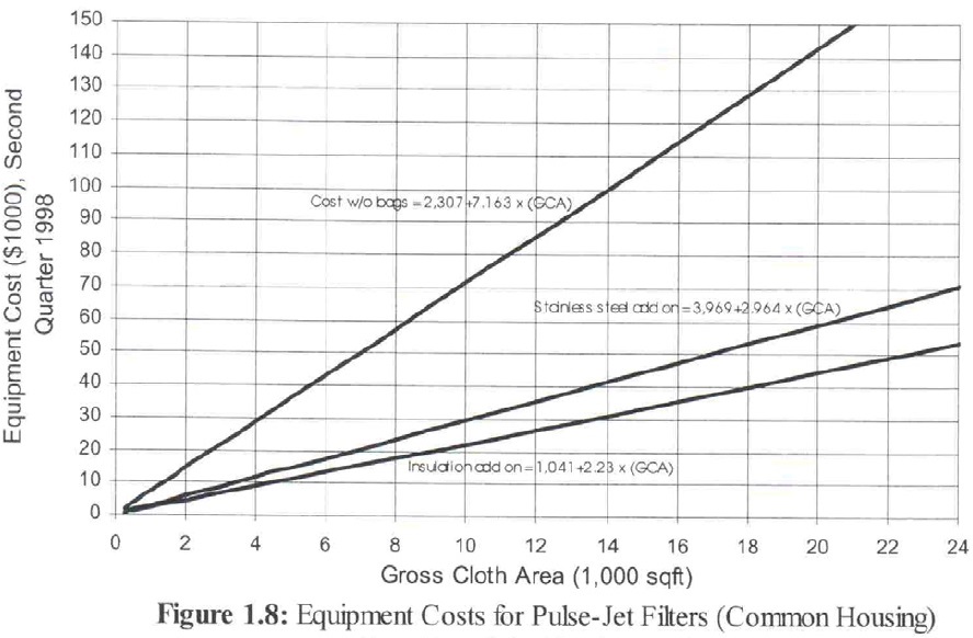
Note: GCA = Gross Cloth Area in square feet.
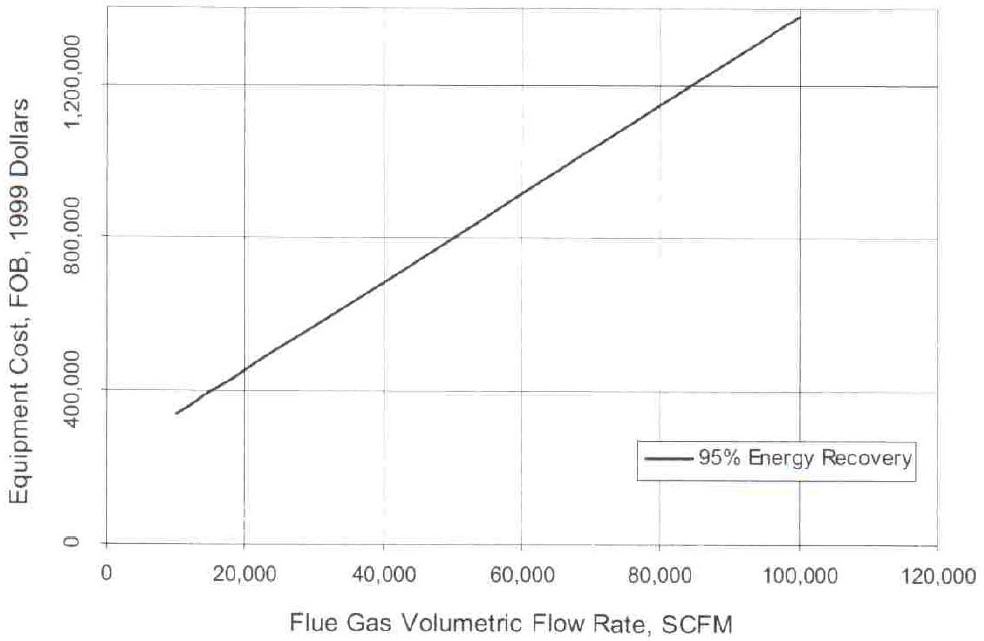
Source: ETS Inc.Graph 2 Typical Data Available for Thermal Oxidizers
- Auxiliary Equipment
This item represents an estimate of the cost of equipment needed to allow the control device to function. This could include components such as hoods/enclosures, ductwork, motors, fans, valves, exhaust stacks, safety by-pass equipment, etc. The OAQPS Control Cost Manual contains formulas and techniques for estimating costs for many of these items. Vendor quotes for supplying control devices often include these items in the direct purchase price and estimates may not be required separately. Auxiliary equipment can typically range from 80 to 120 percent of control device costs with even higher percentages expected as the primary device gets smaller.
- Instrumentation
Often the control device is complex mechanical equipment requiring electronic and/or computerized instrumentation to control. Occasionally, continuous emission monitors or process monitors (temperature, leak detection, etc.) are required and cost estimates are included here. Sometimes instrumentation costs are included with the control device, especially if the cost estimate is from a vendor quote for ‘off-the-shelf’ equipment. Typical cost could be about 10 percent of cost of the control device and auxiliary equipment combined.
- Taxes
Sales taxes apply for most equipment purchases. In Ontario, PST and GST have been estimated at 13 percent of the cost of the control device and auxiliary equipment combined.
- Freight
The cost of shipping equipment needs to be included in the purchased cost estimate. Depending on the size and distance that equipment must be shipped, this can be a significant cost item. Typical costs have been estimated at 5 percent of the cost of the control device and auxiliary equipment combined.
The base price (C) of purchased control equipment is then the sum of items a. through e.
1.7.5.1 Direct Installation Costs
- Foundation and Support
Control devices, ducts, stacks, etc. are often large and heavy requiring addition of structural foundations and supports. Frequently equipment is placed on building roofs requiring installation of reinforced columns and structural steel trusses, etc. Typical costs are estimated at 4 and 8 percent of the base price for filter houses and thermal oxidizers, respectively. Oxidizers being relatively smaller and heavier require slightly more structural support.
- Handling and Erection
Equipment must be delivered, staged and installed. Cranes must be used to move large/heavy components, and welding, bolting and fitting must be completed. Typical costs are estimated at 50 and 14 percent of the base price for filter houses and thermal oxidizers, respectively. Filter houses typically involve far more field construction and fabrication than oxidizers that are largely shop fabricated and shipped ready to install.
- Electrical
Electrical service must be provided and connected to power motors and instruments. This item includes wiring, buses, switches and transformers required to service the control device as well as the electricians to perform the work. Typical costs are estimated at 8 and 4 percent of the base price for filter houses and thermal oxidizers, respectively.
- Piping
Gas lines, stream lines, compressed air, water lines (for the control device and/or fire suppression) and drain lines may be required. Typical costs are estimated at 1 and 2 percent of the base price for filter houses and thermal oxidizers, respectively.
- Insulation
Ductwork and/or piping may require insulation for thermal efficiency or condensation control. Typical costs are estimated at 7 and 1 percent of the base price for filter houses and thermal oxidizers, respectively.
- Painting
Corrosion protection painting of structural elements, some ducts, piping, tanks, control device, etc. may be required. Typical costs are estimated at 4 and 1 percent of the base price for filter houses and thermal oxidizers, respectively.
- Site Preparation
Primarily the related cost associated with clearing obstructions and making space available to receive the new equipment. This is completely site specific and no attempt has been made to estimate routine or customary values. Site specific justification is required to estimate costs here.
- Facilities & Buildings
Occasionally significant ‘infrastructure’ type work is needed to accommodate a new control system. Items such as control device waste handling equipment, boilers to make steam, compressors for air, building additions to house sensitive equipment, etc. Similar to Site Preparation, this is a completely site specific item and no attempt has been made to estimate routine and customary values. Site specific justification is required to estimate costs here.
- Retrofit Costs
Installation of new control equipment into an existing facility can lead to major design and installation changes. Issues such as not enough room to install equipment or special provisions to accommodate available room are related to retrofit. Retrofit costs are not contingencies, which are unexpected costs related to purchasing and installing equipment (addressed elsewhere). Usually carried as a percentage of the total capital cost, USEPA has retrofit costs as high as 30 to 50% for some situations in the OAQPS manual. Higher costs have been used in some MACT standard development documents. Care must be taken in estimating retrofit costs so as to not double count costs. If extra costs are estimated for activities such as foundations, structural supports, erection, electrical, site preparation, facilities & buildings, etc. because of existing conditions then retrofit costs should be correspondingly lower. Site specific justification is required to estimate costs here.
The Total Direct Cost (DC) is then the summation of elements a. through n.
1.7.5.2 Indirect Installation Costs
- Engineering
Design and field support for installation. Typical costs are estimated at 1 percent of the base price for both filter houses and thermal oxidizers.
- Construction and Field Expenses
Costs associated with personnel and miscellaneous costs to fully install and commission the control system. Typical costs are estimated at 20 and 5 percent of the base price for filter houses and thermal oxidizers, respectively. Installation of filter houses is generally a more complicated process because of the greater level of field fabrication involved.
- Contractor Fees
This is contractor profit and is typically estimated to be about 10 percent of the base price of the equipment.
- Start-up
Cost associated with initial placing of the system into operation, adjustments and turn-over of a functioning control system to the facility. Typical costs are estimated at 1 and 2 percent of the base price for filter houses and thermal oxidizers, respectively.
- Performance Test
Testing cost to assure the control device and the system functions as purchased. Compliance testing to demonstrate performance to regulatory agencies may be included in this item. Typical costs are estimated at 1 percent of the base price.
- Contingencies
Provision is provided for unanticipated cost increases. Typical costs are estimated at 3 percent of the base price.
Total indirect costs (IC) are obtained by summing items o. through t.
Total Capital Investment (TCI) = C + DC + IC.
Capital Recovery Cost (CRC) = 0.13587 × TCI. The capital recovery factor is obtained from 6% recovery over a 10-year period and projected as equal uniform annual cash flow of the capital investment, as prescribed in the Ministry’s Guideline for the implementation of Air Standards in Ontario (GIASO).
1.7.6 Annual Operating and Maintenance (O&M) Costs
1.7.6.1 Direct Annual Costs
- Operating Labor (OL)
Estimated hours per year required to operate the POI reduction system or control device multiplied by the hourly operating labor cost. For the simplified example calculation, $30 per hour is used to estimate the hourly labor rate including direct pay and benefits.
- Supervisory Labor (SL)
Annual cost estimate for direct supervision of control system operators should be provided. A reasonable estimate for supervision is obtained by using 15 percent of the operating labor cost and has been applied in the simplified example calculation.
- Maintenance Labor (ML)
Estimated hours per year required to maintain the POI reduction system or control device multiplied by the hourly maintenance labor cost. For the simplified example calculation, $40 per hour is used to estimate the hourly rate for direct pay and benefits which is slightly higher than the operating labor rate to reflect the use of skilled trades.
- Maintenance Materials (MM)
Maintenance of equipment requires the consumption of a wide variety of routine replacement and consumable items such as oil & grease, nuts and bolts, hand tools, washers and gaskets, etc. An estimate of the annual cost for these items is provided here. Typical cost is estimated to be equivalent to maintenance labor cost.
The Direct Labor Cost (D) is then obtained by the summation of elements a. through d.
- Replacement Parts
The purchase of parts and components to replace worn out or broken equipment throughout the life expectancy of the equipment is estimated here. These are items beyond the consumable maintenance materials and include items such as replacement filters for a bag house, heat exchange media for a regenerative thermal oxidizer, spare motors and valves, bearings, VFDs, etc. In addition to larger components that are maintained in facility inventory to shorten repair time, long lead time spare parts may be in this estimate.
- Utilities
An estimate should be provided to quantify the increased consumption of utilities to support operation of the POI reduction technology. These are recurring costs that can represent a significant element in evaluating the appropriateness of a potentially feasible control technique or technology. Generally, estimating utility costs will require a measure of engineering judgment without more detailed design information that is typically not available at the technology evaluation stage. Some examples include;
- Natural Gas – Anticipated annual consumption multiplied by a unit cost. Fuel burning equipment such as thermal oxidizers used to destroy volatile organic contaminants can consume large quantities of natural gas. Based upon the size of a thermal oxidizer determined by the quantity of air flow being controlled a directional estimate of the amount of natural gas required and cost to operate the device may be obtained. For the simplified example calculation it has been assumed that highly efficient thermal recovery devices will be used providing the capability of recovering all but 100°F of the heating value of the oxidizer operation. An estimate of the cost of natural gas has been made at $7.00 per MCF. Similar estimates can be made for other control techniques.
- Compressed Air – Compressed air is required primarily for filter houses, for cleaning filters. The amount of compressed air required is calculated by multiplying the total air flow by the pulse of compressed air required. The simplified example calculation estimated 2 cfm pulse/1000 cfm airflow. The typical cost estimate is $0.25/1000 cfm
- Electricity - Anticipated annual consumption multiplied by a unit cost. Fans are required to move air to and from most control devices and are powered by motors that can consume large amounts of electricity. Other components such as powered dampers and valves and electronic/computer controllers consume electricity, but are generally small relative to motors. Many factors affect the efficiency with which motors consume electricity and detailed engineering is required for proper sizing and design. However, directional estimates can be made. The simplified example calculation estimated 3 hp/1000 cfm of air. The KWH of electricity required were calculated through a simple conversion of hp. The cost estimate used was $0.08 per KWH. It should be noted that 3 hp/1000 cfm may seem high but the cost of running other electrical devices such as powered dampers and valves and electronic/computer controllers were not included.
Total Direct Cost is then the sum of items a. through f.
1.7.6.2 Indirect Annual Costs
- Overhead
Organizational overhead costs for operating labor and maintenance. These are the fixed facility operating costs that increase as the number of employees increase. Typical costs are estimated at about 60% of Direct Labor Costs.
- Administrative Charges
This is an attempt to estimate overhead costs not specifically tied to facility operation such as sales, research and development, accounting, and other home office expenses (not plant overhead). Typically these are estimated at 2% of the projects Total Capital Costs.
- Property Taxes
Fixed assets are normally subject to property taxes. In Ontario, this value has been estimated at 1% of Total Capital Costs which is typically used as an approximation for directional projections.
- Insurance
A simplified estimate for facility and equipment loss protection is obtained with a value of 1% of Total Capital Costs.
Total Annual O&M Costs (OMC) is a sum of indirect and direct annual O&M costs, or a sum of items a. through j.
Total Annual Cost Savings (SAV) is the sum of annual cost savings that may result from implementing a POI reduction technique. Efficiency projects can result in labor and utility reductions or material use savings. These costs should be identified and recorded and the overall cost of the proposal being evaluated reduced equivalently.
1.7.7 Total Annualized Costs
An estimate of the total annual cost (TAC) of purchasing, installing and operating equipment to obtain POI reduction may be obtained by summing the Capital Recover Cost, CRC (i.e. the capital cost spread-out evenly over a 10-year period at a 6% rate of investment return) and annual operating and maintenance cost (OMC) less any cost savings (SAV) identified.
TAC = CRC + OMC − SAV
Annualizing capital cost provides a convenient time frame for combining with operational and maintenance costs which are traditionally planned as yearly recurring expenses. Seasonal variations may also be normalized by using an annual period.
1.7.8 ESDM Information
The total annualized cost of a potential POI reduction technology is to be evaluated relative to a threshold risk reduction cost. Consistent with the Ministry’s risk-based approach to evaluating alteration of air standard requests, the consequence of exposure to a contaminant(s) of concern should be considered in determining the threshold Risk Reduction Cost (RRC).
- Source Emission Before Change
It is important to establish a baseline condition for evaluating potential improvement options. The facility’s ESDM will establish current source conditions resulting in the request for an altered air standard. This value is presented as an annual emission in units of tonnes. The purpose of this value is to establish potential contaminant reduction options on an annual basis consistent with annualized cost estimates.
- Maximum POI Concentration
The facilities dispersion model will predict a maximum POI concentration (POI Cmax) for each contaminant evaluated, this value should be entered on the form. Alternatively, it may be appropriate to use the maximum concentration at a sensitive location, with the approval of the Ministry.
- MOE Standard
The effects-based MOE standard for the contaminant for which the evaluation is being performed should be entered on the form.
- Frequency of Exceedence
The facilities dispersion model will predict the frequency with which the MOE standard would be exceeded based upon operating conditions and the meteorological data set utilized (Note: site specific approved meteorological data must be used to assess frequency of exceedences). The frequency value is expressed as a percentage and should be entered on the form.
- Consequence Score
A consequence score based upon the assignment of a contaminant to a category as defined in information presented in Appendix A to the Ministry’s “Guide to Requesting an Alternative Air Standard” (GRAAS) is entered on the form here. The value will be either 1.43 (Major Health), 1.00 (Medium Health) or 0.86 (Minor Health or Environmental). An explanation regarding derivation of these values may be found in the Risk Scoring section 1.4.2 of this report.
- Risk Quotient
The ratio of maximum POI concentration to the MOE standard is described as the risk quotient and is automatically calculated by the form.
- Risk Score
The risk score for the facility is calculated as the product of Risk Quotient (line f. value), Consequence score (line e. value) and frequency of exceedence (line d. value). The risk score value is automatically calculated by the form.
- Potential POI Improvement
Potential add-on emission control device performance is often expressed as removal efficiency. However, other techniques for reducing contaminant emissions may also be expressed as percent improvements (i.e. material substitutions and process changes), in the technology evaluation stage, estimating performance of a reduction technique may involve approximation of improvement by comparison to other similar sources. Estimation of reduction efficiency across a board range of options is most easily expressed as a percent reduction. Importantly, other source changes that could result in reduction of POI concentrations may be expressed by percent improvement. Source changes such as relocation of exhaust points within a facility can result in significant reduction to projected POI concentrations. While source relocation may not reduce contaminant emissions, its virtual effect may still be expressed as a percent reduction. The estimated percent improvement for the source attributed to the evaluated reduction technique is entered into the form here.
- Equivalent Emission Reduction (or % POI Reduction)
The potential emission reduction of the contaminant(s) reduction technology(s) or technique(s) is simply the product of available emissions (line a. Source Emission before Change) and the reduction potential (line h. Potential POI Improvement). Some POI reduction techniques are not the result of source reductions. Source relocations and exhaust point changes are examples of changes that may reduce POI concentrations without source reduction. However, the POI improvements may still be expressed as virtual reductions for the purposes of evaluating TRE. The value is automatically calculated by the form and entered at line i.
1.7.9 Threshold Risk Reduction Cost (RRC)
A threshold of annualized risk reduction cost is expressed as the product of site specific risk score, site specific contaminant reduction potential and a cost factor. The cost factor used is $10,000 per tonne, which is adjusted upward or downward based upon consequence of potential exposure as expressed by the risk score. The formula is expressed as:
RRC = Risk Score × Potential POI reduction (tonne) × $10,000/tonne
The value is calculated automatically by the form.
1.7.10 Total Resource Effectiveness (TRE) Value
As described previously, the Total Resource Effectiveness Value is determined by the ratio of Total Annualized Cost (TAC) for a potentially feasible POI reduction option to the threshold Risk Reduction Cost (RRC) derived to express the consequence of exposure to a contaminant considering site specific conditions.
The TRE value presents a measure of economic feasibility in close consideration of the consequence of exposure to contaminant(s), using the risk scoring methodologies established in the Ministry’s GIASO document. The TRE methodology provides a consistent approach that is both open and transparent to all stakeholders, for facilities to evaluate cost effectiveness of potentially feasible control options.
1.7.11 Example TRE Value Calculations
Application of the total resource effectiveness calculation methodology may be best illustrated through example. With relatively limited source information, creditable estimates may be derived to evaluate the effectiveness of resource utilization in achieving POI reductions. The source information is readily available from a facility’s ESDM report. Potential POI reduction techniques are identified through the facility’s Technology Benchmarking Review. Cost information may be obtained from a variety of sources. USEPA's Control Cost Manual provides a wealth of information needed to estimate the cost of a wide range of add-on emission control devices. Other sources (i.e. engineering texts, trade publications, research publications, etc.) may also provide useful information. Vendor quotes to provide equipment and/or service can provide the highest quality cost information, but may be the most difficult to obtain when performing feasibility evaluations. Most importantly, engineering judgment is required throughout the process of assembling information and costing potential POI reduction techniques. Forms that add structure and format to assembling and presenting cost effectiveness information can aid (but not replace) the environmental professional’s judgment.
Three (3) example calculations will be presented to help illustrate the application of the TRE methodology and use of the indicator value to aid evaluation of potential POI reduction techniques. The first two examples evaluate the appropriateness of installing add-on control devices to reduce emissions. The first source is evaluated for particulate emission reduction and the other source for volatile organic compound reduction. The third example will illustrate how the methodology may be utilized to evaluate a process change as a potential POI reduction technique.
Example 1
A facility operates a process that generates a significant quantity of particulate emissions. The facility has provided the process with a hood and ventilation system to capture fumes and direct them to an existing filter house to reduce particulate emissions. In this example we utilize available information to evaluate the reasonableness of the facilities decision to install and operate the emission control device using the TRE methodology. This example provides an opportunity to ‘ground truth’ the TRE methodology and indicator value versus existing decision making.
From the facility’s ESDM it is determined that the source exhausts 0.1 g/s of particulate material contained in 57,000 cfm of process air. The facility intends to operate the source without restriction (i.e. 8,760 hours per year). For this example, it will be assumed that the facility is exceeding the TSP standard of 100 µg/m3 and operating in the mid-ALARA region (i.e. 5 times the standard, 50% of the time).
Refer to Figure 1 in Attachment 1 to see how the calculations proceed when the information is entered. Data entered into the form is highlighted in blue for clarity. Those values not in blue are automatically generated by the form.
Turning to USEPA's Control Cost Manual, Section 6, Chapter 1 Particulate Controls for assistance with estimating control costs the following calculations are performed.
Control Device
Based upon the source to be controlled and engineering judgment it is decided to evaluate a pulse jet type filter house operated under positive pressure using fiberglass filters. In addition, it is assumed that the exhaust air temperature will be below 500°F, so no pre-filter cooling is required. Further, a gas to cloth ratio of 6 will be assumed to approximate the filter area required. Other filter types, materials and ratios could be chosen, but these have been selected for this evaluation. So, initial filter house sizing is determined by the following calculation;
57,000 cfm/6 (gas to cloth ratio) = 9,500 sq. ft. × 1.5 (Table 1.2) = 14,250 sq. ft.
{Table 1.2 values are used to convert net filter area to gross or required surface area.}
Next, using regression formulas derived from actual cost data collected by USEPA, an estimate of the pulse-jet filter house control device cost may be calculated.
From Figure 1.8, Pulse-Jet Filters (Common Housing);
Filter house cost − 2,307 + 7.163(14,250) = $ 104,380
Added cost for stainless steel construction − 3,696 + 2.964(14,250) = $45,933
{Stainless steel construction is selected for durability given the source being evaluated}
From Table 1.8: Bag Prices - Fiberglass filters using bottom bag removal, $1.69/ft2;
14,250 × 1.69 = $24,083
Further, from Table 1.8: Bag Prices – Assume stainless steel cages 5 1/8 inches × 10 feet;
5 1/8 inches / 12 × 3.14 × 10 = 13.4 sq. ft./cage
14,250/13.4 = 1,063 cages required
[8.8486 + 1.2284(13.4)] × 1,063 = $26,904
An estimate of the control device cost is then the sum of these four values;
104,380 + 45,933 + 24,083 + 26,904 = $201,300
Auxiliary Equipment
The control device cannot reduce TSP emissions without a fume capture hood, ventilation ducts, fans, motors and exhaust stack. Cost estimates can be made for these elements by using regression formulas contained in USEPA's Control Cost Manual, Section 2, Chapter 1. The following cost calculations are performed;
Fume Capture Hood
From Equation 1.40,
C = aAfb
Where,
- C
- Cost ($)
- a
- 306 - Table 1.8 Canopy rectangular
- b
- 0.506 - Table 1.8 Canopy rectangular
- Af
- Face area of hood (ft2) = air flow (cfm)/500 fpm
{500 fpm is selected to achieve suitable fume capture velocity}
This cost estimate is not used for this example since an existing hood is in place yielding the reported capture efficiency and emission rate. Making a change to the basic capture system design would introduce undesirable inaccuracy to the ESDM reported emission information for this example. The existing capture hood will be assumed to remain in service.
Ventilation Duct
From Equation 1.40,
C = aDb
Where,
- C
- Cost per foot of duct ($)
- a
- 1.56 - Table 1.9, stainless steel circular
- b
- 1.00 - Table 1.9, stainless steel circular
- D
- Duct diameter (inches) = air flow (cfm)/4,000 fpm
{4,000 fpm is selected to keep PM suspended in duct}
Then,
57,000/4,000 = 14.25 sq. ft.
Diameter = SQRT[(4 × 14.25)/3.14] = 4.3 feet or about 52 inches
1.56(52)1.0 × 100 feet = $8,112
{100 feet of duct assumed for this example}
Duct Elbows
From Equation 1.41,
C = aebD
Where,
- C
- Cost per elbow ($)
- a
- 74.2 - Table 1.10, stainless steel elbows
- b
- 0.0668 - Table 1.10, stainless steel elbows
- D
- Duct diameter (inches)
Then,
74.2e(0.0668 × 52) × 4 = $9,573
{4 elbows assumed for this example}
Ventilation Dampers
From Equation 1.41,
C = aDb
Where,
- C
- Cost per damper ($)
- a
- 208 - Table 1.10, Aluminized CS louvered with actuators
- b
- 0.791 - Table 1.10, Aluminized CS louvered with actuators
- D
- Duct diameter (inches)
Then,
74.2e(0.0668 × 52) × 4 = $9,573
{4 elbows assumed for this example}
Stack
From Equation 1.41,
C = aDbL
Where,
- C
- Cost ($)
- a
- 12.0 - Table 1.12, Plate stainless steel
- b
- 1.20 - Table 1.12, Plate stainless steel
- D
- Stack diameter (inches)
{3,000 fpm stack exhaust velocity assumed for proper dispersion,
57,000/3,000 = 19 sq.ft.
Then,
- D
- SQRT[(4 × 19)/3.14] = 4.9 feet or about 60 inches}
- L
- Stack height (feet)
Then,
12(60)1.20 × 50 = $81,646
{50 feet tall stack assumed for this example}
Motors and Fans
Using engineering judgment, an estimate of the cost of providing two fans and motors to power the capture hood and ventilation system and exhaust air from the filter house is made. More detailed cost estimating could be provided based upon fan type, duct runs, friction losses, pressure drop as well as motor types and energy curves and other considerations. However, the added effort required would probably not significantly improve the value of the overall cost estimating evaluation.
Then,
Motors & Fans = $50,000
An estimate of the auxiliary equipment cost is then the sum of these five values;
8,112 + 9,573 + 9,472 + 81,646 + 50,000 = $158,803
We now have enough information to complete a calculation of estimated total resource effectiveness for the add-on TSP control device. Using the template form for a Fabric Filter previously prepared, the source information collected from the facility’s ESDM and equipment costs estimated above, we may enter information into the form to complete the calculations. The Fabric Filter form contains typical values determined by USEPA based upon review of extensive cost information collected from installation of similar devices that are used to complete the estimate of the base equipment cost, direct and indirect installation costs and operating and maintenance costs. Ontario specific values have been included where appropriate to reflect costs associated with taxes, labor and utilities. Line-by-line review of the cost estimates by an environmental professional is necessary to establish the reasonableness of the estimates to the facility specific circumstances being evaluated.
Upon entering the Fabric Filter form, source information is entered to enable automated estimates of certain operating costs to be calculated. The source air flow (i.e. 57,000 acfm) and operating hours (i.e. 8,760 hours) are entered into the designated ‘boxes’ near the top of the form. Then values are added based on the calculations performed above to capture ‘Purchased Equipment Costs’, line a. ‘Control Device’ (i.e. $201,300) and line b. ‘Auxiliary Equipment’ (i.e. $158,803). Typical values for line c. ‘Instruments & Controls’, line d. ‘Sales taxes’, and line e. ‘Freight’ are automatically calculated.
Review of the default Purchased Equipment Cost values appears reasonable and they will be used. Instruments & controls have been estimated at 10% of combined control device and auxiliary equipment costs and reflect the cost of pressure and temperature monitors, perhaps a leak detection system, and VFD damper and motor controls. PST and GST taxes are estimated at 13% for Ontario and the cost of shipping control components from the manufacturing site to the installation facility is estimated at 5%. Freight is an obvious candidate for revision from the default value since shipping distance will directly and significantly affect cost. For this example the default value is accepted.
The Base Price (C) is automatically calculated by summing values from line a. through e.
Direct Installation Costs
Automated cost estimates continue to be calculated for Direct Installation Costs with typical values assigned as a ratio of the Base Price (C) determined for the purchased equipment. These represent costs directly associated with preparing, placing, connecting and otherwise installing the control device ready for operation. Typically, filter houses are installed on building roofs roughly above the source to be controlled if possible. Structural supports to hold the additional weight of the control system must be provided including platform, trusses, columns and foundations. These elements are estimated by line f. ‘Foundation’ at 4% of the base equipment price. This value could be significantly higher depending on site specific circumstances or lower if placing on the ground requiring only duct support and a concrete pad. The default value will be used for this example.
Line g. ‘Handling & Erection’ represents the bulk of the installation costs and represents staging, placing, connecting and installing all pollution control device related equipment. In this example, it is assumed that cranes would be used to lift structural members, duct work, stack, filter house, etc. to roof level for installation. Welding and bolting of components using skilled trades for rigging and welding etc. A typical cost estimate of 50% of the base equipment price appears reasonable for this example and has been used. Special circumstances can drive the cost higher such as needing helicopter lifts or staging to avoid production disruptions (lifting equipment over occupied building is generally not allowed).
Cost estimates for providing electrical connections including primary power supply and component wiring using skilled trade electricians is provided in line h. ‘Electrical’ and estimated at 8% of base equipment price. Site specific conditions could cause costs to be higher for this item such as the need for new transformers, switches or busses to provide power to the control device. This is not the case for the current example and the typical values will be used.
Plumbing and other pipe connections to the control system are estimated at 1% of the base equipment cost. Line i. ‘Piping’ includes cost associated with supplying water, compressed air and condensate drains required to make the TSP control system functional. Other costs such as natural gas piping and fire suppression could be included in this item for other control systems.
Thermal efficiency and condensation protection are important considerations for control systems especially in cold weather climates. Provision for ‘Insulation’ of air ducts and pipes is estimated at 7% of the base equipment cost in line j. The filter house is usually provided with insulation by the device supplier, but if required insulation is not provided then a cost estimate may be include in this line item. The typical fraction determined by USEPA will be used for this example.
Painting to provide corrosion protection and system durability is an important consideration. Line k. ‘Painting’ is provided to capture costs associated with application of functional coatings and is estimated at 4% of the base equipment cost. For this example, stainless steel has been specified for the filter house, air ducts and stack making painting of these elements unnecessary. However, painting of structural and support elements remain an important aspect to assure system durability and the 4% typical estimate does not appear to be excessive for this work and will be retained for the example.
Direct installation costs may involve activities that are completely unique to the site being evaluated and are therefore difficult to estimate using ‘typical’ factors obtained by comparing to similar installations. Items such as ‘Site Preparation’, ‘Facilities & Buildings’, and ‘Retrofit Costs’ should be considered by the environmental professional familiar with the site and installation requirements in estimating direct installation costs. Space is provided in the form (lines l, m & n) to include cost values as appropriate for these items.
Site preparation relates to the range of activities required to prepare the site for installation of the TSP control system and associated equipment. Site preparation could include ground clearing and leveling, building demolition, equipment removal, changes to existing roadways, parking, fencing and other existing features that must be rearranged to make access for the new equipment possible. For this example, it is assumed that no such site preparation is required.
Occasionally, installation of a control device involves the construction of new building(s) to house equipment. This could be in the form of a penthouse type structure erected on the roof of an existing building to provide weather protection for control equipment or a grade level building adjacent to the existing facility. Building is usually associated with larger, more extensive control systems. For this example, no building additions are projected.
Similarly, additional support facilities may be required to operate the control device. For the pulse jet type filters being evaluated in this example, compressed air is required to periodically remove particulate matter collected on the fiberglass filters. If the facilities capability to supply compressed air needs to be expanded (or provided) to accommodate the new equipment, then new ‘facilities’ must be added in the form of air compressor(s). Other control systems may involve handling waste water in terms of treatment and disposal. Still other control systems may involve handling special chemicals and hazardous waste that would involve additional ‘facilities’. All of these special ‘facility’ actions should be estimated and included in the direct installation cost. For this example, no special facility costs have been identified.
Additional site specific and unique requirements associated with ‘retrofitting’ control measures to existing facilities can add significant costs to installation. Provision is made in the form at line n. for ‘Retrofit Costs’. These are costs unique to the site and source that make installation more difficult and costly. Retrofit can be relatively difficult and subjective costs to estimate, but relate to things like space constraints, clearances and rearrangements required to install the equipment. Hoods, enclosures and ducts may be more difficult to place and existing equipment may need to be moved or changed to provide required access. Additional costs associated with retrofitting controls on existing equipment will almost always occur and can range from only a couple percent of the base equipment cost to as much as 1 or 2 times purchased equipment costs. Retrofit factors up to 50% of the base equipment cost are not unlikely and that is the amount used for this example.
In general, the larger and more complex the project, the greater the retrofit cost that should be expected. The environmental professional’s knowledge of the facility and equipment is critical in developing reasonable estimates for this cost element. Care should be taken to not double count costs. If extraordinary costs are projected for individual installation items such as additional structural steel, foundations, erection complexities, extra long duct, pipe and electrical runs, additional transformers, etc. in lines f. through m., then perhaps separately identified retrofit costs might be correspondingly lower. In addition, retrofit costs should not be thought of as contingency (those will be addressed separately). Retrofit costs should be anticipated and planned for while contingency costs would result from unanticipated events.
Total Direct Costs (DC) is then the summation of line items f. through n.
Indirect Installation costs
There are additional costs associated with installation of the TSP control system and result in indirect expenditures. The Fabric filter form automatically calculates values in line items o. through t. providing estimates for these indirect costs based upon typical rates determined by USEPA's survey of equipment suppliers and installations. For this example, the typical values will be used.
Line item o. ‘Engineering & Supervision’ represents the cost of system design and engineering supervision of field work. This item is estimated at 1% of the base equipment cost and appears reasonable. Line item p. ‘Construction & Field Expenses’ represents a kind of ‘catch-all’ for costs associated with getting the equipment installed and functioning. These include incidental costs related to construction and services, equipment and supplies obtained on-site to complete installation. Estimated at 20% of base equipment cost, it is accepted as a reasonable value for this example.
Contactor profit is reflected in line q. ‘Contractor Fees’ and is estimated at 10% of base equipment cost. Initial ‘Start-up’ is addressed at line r. and is estimated to be 1% of base equipment cost. Typically, equipment is not ‘turned over’ to the facility until operation consistent with the contract guarantee has been established. Start-up costs represent this initial trial operation. Closely related to start-up costs are ‘Performance Tests’ provided at line s. Initial performance tests are typically required to certify to the facility that TSP removal efficiencies are being achieved, as advertised. Other types of testing such as energy and pressure performance may also be specified. This item is estimated at 1% of base equipment cost. However, if system compliance testing is required to demonstrate to regulatory agencies performance levels achieved, then additional cost projections would likely be appropriate. The certification testing estimated for this example is $4,409. Compliance testing using approved test methods by independent professional services could cost $20,000 or more.
The last element of indirect installation cost estimating is to provide for unforeseen expenditures required to support completion of the project. A small estimate for ‘Contingencies’ of 3% of base equipment cost is provided at line t. for unanticipated occurrences such as labor disputes, stainless steel price increases, weather delays, etc.
The Total Indirect Costs (IC) is then determined by summation of line items o. through t.
Total Capital Cost (TCI) to purchase and install a pulse jet TSP filter system at the example facility is then estimated by the summation of Base Price (C), Total Direct Costs (DC) and Total Indirect Costs (TCI). The form automatically tallies the values.
The total capital cost represents a one-time investment in control technology over the life of the equipment. It is desirable to convert the total capital cost to equal annualized cost for the purpose of completing the evaluation of the total resource effectiveness of the potential control measure considered in this example. Using the amortization period of 10 years and interest rate of 6% provided in Section 2.5 of the Ministry’s GIASO document, the following multiplier is calculated.
i / {1 − (1 + i)-n}
Where,
- i
- 6 % interest rate
- n
- 10 year equipment life
Then,
0.06 / {1 − (1 + 0.06)-10} = 0.13587
The Capital Recovery Cost (CRC) is automatically calculated in the Fabric Filter form by multiplying Total Capital Costs (TCI) by the annualizing factor above.
Annual Operating and Maintenance (O&M) Cost
The example now proceeds to estimate costs associated with operating and maintaining the TSP control system. The Fabric Filter form automates many of the required cost estimates to simplify the calculations needed. The environmental professional performing the evaluation should review each line item to judge the reasonableness of the value for the specific source and site being considered. Similar to capital costs, operating O&M costs may be both direct and indirect.
Running the TSP control system requires personnel to start-up, shut-down and attend to the equipment during operation. Line a. ‘Operating Labor’ provides an estimate of cost based upon an hourly rate of $30/hour and an estimate that 2-hours per production shift is required to attend to the system. The 2-hour per shift estimate comes from USEPA survey of typical operating requirements for similar systems. Other estimates may be appropriate, but these values are judged to be reasonable for this example.
All operating personnel require supervision to schedule and direct activities. Line b. ‘Supervisor Labor’ provides and estimate for supervision as a faction (15%) of operating labor cost. The factor comes from USEPA's survey of similar TSP control systems and is accepted as reasonable for this example.
In addition to operating the TSP control system, maintenance also requires personnel. Line c. ‘Maintenance Labor’ provides an estimate of cost based upon an hourly rate of $40/hour and an estimate of 1-hour per production shift (on average) to maintain the equipment. Again, the time estimate comes from USEPA's survey of typical maintenance required for similar systems. Other estimates may be appropriate, but these values are judged to be reasonable for this example.
Routine maintenance usually involves the consumption of a variety of materials ranging from oil & grease, nuts & bolts and rags to hand tools such as wrenches and screw drivers. Line d. ‘Maintenance Materials’ is provided to estimate these costs and are typically considered to be about equivalent to the cost of maintenance labor.
Direct Labor Costs (DC) is then the summation of lines a. through d.
There are other direct operating costs in addition to labor. These are costs associated with maintaining spare parts, routine replacement parts/components, utilities, bulk material s, and waste disposal. The environmental professional must consider the potential POI reduction technique being evaluated and include the appropriate items in the cost estimate. For this example of a TSP control system it has been determined that replacement parts, compressed air and electricity would be required to operate the system. The Fabric Filter form identifies these items and provides automated estimates for the utilities to aid completion of the TRE calculation.
First, the form makes provision for ‘Replacement Parts’ at line e. and this is intended to reflect the need to periodically replace the fiberglass filters. For this example, it has been assumed that all the filters will need to be replaced every two years. Consequently, half the cost of providing all new fiberglass filters (see the initial equipment cost calculations above, Device Cost). Other estimates could be made, but this seems reasonable for typical fabric filter use.
Next, ‘Compressed Air’ is required to regularly ‘blow-off’ particulate matter accumulated on the filter surface. Provision for an estimate is provided at line f.
and an automatic calculation is provided in the Fabric Filter form based upon the following equation;
(air flow, cfm) × (operating hours) × 60 min/hr × 2 cfm pulse/1000 cfm air flow × $0.25/1000 cfm
Where,
- Air flow
- 57,000 cfm for this example
- Operating hours
- 8.760 hours per year for this example
- 2 cfm/1000 cfm air flow
- Typical air pulse required to remove particulate matter from filter surface
- $0.25/1000 cfm
- Typical cost to provide compressed air
Then,
57,000 × 8,760 × 60 × 2/1,000 × 0.25/1,000 = $14,980
Electricity is also required to power the TSP control system. An estimate of electricity required is provided at line g. ‘Electricity’ and an automatic calculation is performed in the Fabric filter form based upon the following equation;
(airflow, cfm) × (operating hours) × 3 hp/1000 cfm × 0.746 kWh/hp/$0.08/kWh
Where,
- Air flow
- 57,000 cfm for this example
- Operating hours
- 8.760 hours per year for this example
- 3 hp/1,000 cfm
- Typical power required to move 1,000 cfm of air
- 0.746 kWh/hp
- Conversion of power to energy
- $0.08/kWh
- Estimate of electricity cost in Ontario
Then,
57,000 × 8,760 × 3/1,000 × 0.746 × 0.08 = $59,599
There are other indirect operating costs that may not be immediately apparent but should be considered. Fortunately, there are typical factors that have been developed by USEPA based upon extensive review of similar control device installations that may be used to provide cost estimates.
‘Overhead’ at line h. allows for the cost associated with facility related organizational overhead to be provided. This has been estimated at 60% of Direct Labor Costs (D), is automatically calculated in the Fabric Filter form and has been accepted as reasonable for this example.
Non-facility or operational related costs such as sales & marketing, R&D, accounting, and other ‘home office’ type costs may be estimated at line i. ‘Administrate Charges’ and are automatically calculated in the Fabric Filter form using 2% of Total Capital Cost (TCI).
‘Property Taxes’, line j. and ‘Insurance’, line k. are both estimated at 1% of Total Capital Cost (TCI). Other values could be used, but these are considered representative for this example.
Total Annual O&M Costs (OMC) may be obtained by the summation of lines a. through k. and is automatically calculated by the Fabric Filter form.
Occasionally, a POI reduction technique results in cost savings to the facility (perhaps through energy reduction or material use efficiencies). Provision is provided in the form to estimate savings that would effectively reduce the annual operating cost of implementing the POI reduction technique. This is not the case in this example and no operational savings have been identified.
Similarly, Some POI reduction techniques may result in the recovery or production of a valuable by-product that could become a revenue stream for the facility. Provision is provided in the form to estimate potential revenues that would effectively reduce the annual operating cost of implementing the POI reduction technique. This is not the case in this example and no new revenue has been identified.
The Total Annualized Costs (TAC) is then the summation of Capital Recovery costs (CRC), Total Annual O&M Costs (OMC), Total Annual Savings (SAV), and Total Annual Revenue (REV). This value is automatically calculated in the Fabric Filter form.
The total resource effectiveness value may now be calculated by entering ESDM information into the Fabric filter form. Calculations will automatically be completed upon entry of the required data to generate the final TRE value.
ESDM Information
Line a. ‘Source Emission Before Change’ requires the entry of annual emission from the source being evaluated of the substance of interest. The value should be entered in units of tones per year. This may require converting grams per second emission rate contained in the sites ESDM. For this example the following calculation is performed to estimate the ‘before control’ emission rate.
{(0.1 g/s) × (0.002205 lbs/g) × (3,600 s/hr) × (8,760 hr/yr)}/ (2,200 lbs/tonne) × (1 − 0.99 % control) = 316 tonnes per year
The TSP emission rate and operating hours come directly from the site’s ESDM. For this example, we are evaluating the decision already made to install and operate a TSP control device so an estimate has been made of current performance level (i.e. 99% effective at removing TSP).
The ‘POI Concentration’ at the maximum off-site location (or the agreed to sensitive receptor) obtained from the site’s ESDM report is entered at line b. For this example, it is assumed that the maximum POI is five times the TSP standard (i.e. 500 µg/m3). The ‘MOE Standard’ is entered at line c. and for this example evaluating a TSP control option, the value is 100 µg/m3.
The ‘Frequency of Exceedance’ as determined by the site’s ESDM report at the POI agreed to with the Ministry (i.e. maximum or sensitive receptor) and is entered at line d. For this example, 50% frequency of exceedance is assumed based upon a mid-ALARA region occurrence.
The ‘Consequence Score’ is determined based upon the contaminant being evaluated and the GIASO designated ranking regarding health and/or environmental effect. For this example, TSP represents a medium health effect substance and is therefore assigned a consequence score of 1.00 and the value is entered at line e.
Automated calculations are now performed in the Fabric Filter form to determine the sites ‘Risk Quotient’ (RQ), line f. and ‘Risk Score’ (R), line g. These values are derived from the site specific information entered in lines b. through e. The formulas are displayed on the form.
The last data point to be entered into the form relates to the ‘Potential POI Improvement’ that may be provided by the reduction technique being evaluated. The percentage reduction possible at the source being evaluated should be entered at line h. For an add-on control measure, this value is effectively the control efficiency possible expressed as a percentage. A pulse jet type fabric filter should be capable of achieving 99% removal of particulate matter and this value has been used. In other circumstances there could conceivably be source changes that do not actually reduce emissions but effectively reduce the sources POI contribution (i.e. exhaust stack location changes). These improvements should be reflected as ‘virtual’ emission reductions equivalent to the anticipated POI improvement.
The Total Resource Effectiveness (TRE) Value is automatically calculated in the Fabric Filter form from the information entered and displayed in a ‘box’ at the bottom of the page. Intermediate calculations of the ‘Equivalent Emission Reduction’ value is automatically calculated and displayed at line i. as an effective contaminant reduction in terms of tonnes per year. Similarly, a ‘Threshold Risk Reduction Cost’ (RRC) is calculated based on the product of Risk Score, Potential Emission Reduction and cost index of $10,000.
The TRE values provide an indication of the relative effectiveness of potential POI reduction techniques. TRE values less than 1.0 would generally indicate a reasonably effective use of resources to achieve the potential POI improvement. However, TRE values above 1.0 and ranging up to about 10.0 may suggest further consideration is appropriate and/or refinement of assumptions are required. TRE values over 10.0 would generally indicate the potential POI reduction technique is not a good use of resources and perhaps other options should be considered. For this example, a TRE value of 0.07 is determined. This result suggests that the facilities decision to install the TSP control device appears to be a good choice and represents an effective use of resources.
Concluding Comments
The judgment of an environmental professional is required to effectively complete a Total Resource Effectiveness calculation. Standardized format and automated calculations can facilitate and speed the process. Engineering estimates and judgment will be required even with the best data available. The forms provide considerable space to annotate comments and append foot notes for the environmental professional to explain how values are created and assumptions made. Fully using comments and foot notes to explain judgments and assumptions will significantly improve the transparency of the process and enhance the acceptability of the evaluation.
Example 2
A facility operates a process that generates a significant quantity of volatile emissions. The source is enclosed and exhausted outside the manufacturing building. In this example we utilize available information to evaluate the reasonableness of installing and operating an emission control device using the TRE methodology.
From the facility’s ESDM it is determined that the source exhausts 0.8 g/s of volatile material contained in 110,000 cfm of process air. The facility intends to operate the source without restriction (i.e. 8,760 hours per year). For this example, it will be assumed that the facility is exceeding a volatile substance standard of 0.08 µg/m3. Further, the facility’s ESDM indicates the maximum POI concentration to be 1.80 µg/m3 and exceeds the standard at this point 33.8% of the time.
Refer to Figure 2 in Attachment 1 to see how the calculations proceed when the information is entered. Data entered into the form is highlighted in blue for clarity. Those values not in blue are automatically generated by the form.
Turning to USEPA's Control Cost Manual, Section 6, Chapter 2 VOC Controls for assistance with estimating control costs the following calculations are performed.
Control Device
Based upon the source to be controlled and engineering judgment it is decided to evaluate a regenerative thermal oxidizer. Using regression formulas derived from actual cost data collected by USEPA, an estimate of the pulse-jet filter house control device cost may be calculated.
From Figure 2.5, thermal Incinerators, Regenerative;
RTO cost − 2.204×10⁵ + 11.57(110,000) = $1,493,100
Auxiliary Equipment
The control device cannot reduce volatile emissions without ventilation ducts, fans, motors and exhaust stack. Cost estimates can be made for these elements by using regression formulas contained in USEPA's Control Cost Manual, Section 2, Chapter 1. The following cost calculations are performed;
Ventilation Duct
From Equation 1.40,
C = aDb
Where,
- C
- Cost per foot of duct ($)
- a
- 1.56 - Table 1.9, stainless steel circular
- b
- 1.00 - Table 1.9, stainless steel circular
- D
- Duct diameter (inches) = air flow (cfm)/4,000 fpm
{4,000 fpm is selected to keep PM suspended in duct}
Then,
110,000/4,000 = 27.5 sq. ft.
Diameter = SQRT[(4 × 27.5)/3.14] = 5.9 feet or about 72 inches
1.56(72)1.0 × 100 feet = $ 11,232
{100’ of duct assumed for this example}
Duct Elbows
From Equation 1.41,
C = aebD
Where,
- C
- Cost per elbow ($)
- a
- 74.2 - Table 1.10, stainless steel elbows
- b
- 0.0668 - Table 1.10, stainless steel elbows
- D
- Duct diameter (inches)
Then,
74.2e(0.0668 × 72) × 4 = $36,412
{4 elbows assumed for this example}
Ventilation Dampers
From Equation 1.41,
C = aDb
Where,
- C
- Cost per damper ($)
- a
- 208 - Table 1.10, Aluminized CS louvered with actuators
- b
- 0.791 - Table 1.10, Aluminized CS louvered with actuators
- D
- Duct diameter (inches)
Then,
208(72)0.791 × 2 = $12,253
{2 dampers assumed for this example}
Stack
From Equation 1.41,
C = aDbL
Where,
- C
- Cost ($)
- a
- 12.0 - Table 1.12, Plate stainless steel
- b
- 1.20 - Table 1.12, Plate stainless steel
- D
- Stack diameter (inches)
{3,000 fpm stack exhaust velocity assumed for proper dispersion, 110,000/3,000 = 36.7 sq.ft.
Then,
D = SQRT[(4 × 36.7)/3.14] = 6.8 feet or about 82 inches}
- L
- Stack height (feet)
This cost estimate is not used for this example since an existing stack is in place meeting good engineering standards. The existing stack will be assumed to remain in service.
Motors and Fans
Using engineering judgment, an estimate of the cost of providing two fans and motors to power the capture hood and ventilation system and exhaust air from the filter house is made. More detailed cost estimating could be provided based upon fan type, duct runs, friction losses, pressure drop as well as motor types and energy curves and other considerations. However, the added effort required would probably not significantly improve the value of the overall cost estimating evaluation.
Then,
Motors & Fans = $100,000
An estimate of the auxiliary equipment cost is then the sum of these four values;
11,232 + 36,412 + 12,253 + 100,000 = $159,897
We now have enough information to complete a calculation of estimated total resource effectiveness for the add-on volatile control device. Using the template form for an Oxidizer – Thermal Regenerative previously prepared, the source information collected from the facility’s ESDM and equipment costs estimated above, we may enter information into the form to complete the calculations. The Oxidizer – Thermal Regenerative form contains typical values determined by USEPA based upon review of extensive cost information collected from installation of similar devices that are used to complete the estimate of the base equipment cost, direct and indirect installation costs and operating and maintenance costs. Ontario specific values have been included where appropriate to reflect costs associated with taxes, labor and utilities. Line-by-line review of the cost estimates by an environmental professional is necessary to establish the reasonableness of the estimates to the facility specific circumstances being evaluated.
Upon entering the Oxidizer – Thermal Regenerative form, source information is entered to enable automated estimates of certain operating costs to be calculated. The source air flow (i.e. 110,000 acfm) and operating hours (i.e. 8,760 hours) are entered into the designated ‘boxes’ near the top of the form. Then values are added based on the calculations performed above to capture ‘Purchased Equipment Costs’, line a. ‘Control Device’ (i.e. $1,493,100) and line b. ‘Auxiliary Equipment’ (i.e. $159,897). Typical values for line c. ‘Instruments & Controls’, line d. ‘Sales taxes’, and line e. ‘Freight’ are automatically calculated.
Review of the default Purchased Equipment Cost values appears reasonable and they will be used. Instruments & controls have been estimated at 10% of combined control device and auxiliary equipment costs and reflect the cost of pressure and temperature monitors, perhaps a leak detection system, and VFD damper and motor controls. PST and GST taxes are estimated at 13% for Ontario and the cost of shipping control components from the manufacturing site to the installation facility is estimated at 5%. Freight is an obvious candidate for revision from the default value since shipping distance will directly and significantly affect cost. For this example the default value is accepted.
The Base Price (C) is automatically calculated by summing values from line a. through e.
Direct Installation Costs
Automated cost estimates continue to be calculated for Direct Installation Costs with typical values assigned as a ratio of the Base Price (C) determined for the purchased equipment. These represent costs directly associated with preparing, placing, connecting and otherwise installing the control device ready for operation. Typically, thermal oxidizers are installed on building roofs roughly above the source to be controlled if possible. Structural supports to hold the additional weight of the control system must be provided including platform, trusses, columns and foundations. These elements are estimated by line f. ‘Foundation’ at 8% of the base equipment price. This is a large RTO and would likely be placed at ground level on a concrete pad instead of installed on the roof. However, the large size of this RTO would likely off-set any savings obtained by not placing the unit on the roof. The default value will be used for this example.
Line g. ‘Handling & Erection’ represents the bulk of the installation costs and represents staging, placing, connecting and installing all pollution control device related equipment. In this example, it is assumed that cranes would be used to lift structural members, duct work, RTO, etc. to roof level for installation. Welding and bolting of components using skilled trades for rigging and welding etc. A typical cost estimate of 14% of the base equipment price appears reasonable for this example and has been used.
Cost estimates for providing electrical connections including primary power supply and component wiring using skilled trade electricians is provided in line h. ‘Electrical’ and estimated at 4% of base equipment price. Site specific conditions could cause costs to be higher for this item such as the need for new transformers, switches or busses to provide power to the control device. This is not the case for the current example and the typical values will be used.
Plumbing and other pipe connections to the control system are estimated at 2% of the base equipment cost. Line i. ‘Piping’ includes cost associated with supplying natural gas, fire suppression water and condensate drains required to make the RTO control system functional.
Thermal efficiency and condensation protection are important considerations for control systems especially in cold weather climates. Provision for ‘Insulation’ of air ducts and pipes is estimated at 1% of the base equipment cost in line j. The RTO is usually provided with insulation by the device supplier, but if required insulation is not provided then a cost estimate may be include in this line item. The typical fraction determined by USEPA will be used for this example.
Painting to provide corrosion protection and system durability is an important consideration. Line k. ‘Painting’ is provided to capture costs associated with application of functional coatings and is estimated at 1% of the base equipment cost. For this example, stainless steel has been specified for the RTO and air ducts making painting of these elements unnecessary. However, painting of structural and support elements remain an important aspect to assure system durability and the 1% typical estimate does not appear to be excessive for this work and will be retained for the example.
Direct installation costs may involve activities that are completely unique to the site being evaluated and are therefore difficult to estimate using ‘typical’ factors obtained by comparing to similar installations. Items such as ‘Site Preparation’, ‘Facilities & Buildings’, and ‘Retrofit Costs’ should be considered by the environmental professional familiar with the site and installation requirements in estimating direct installation costs. Space is provided in the form (lines l, m & n) to include cost values as appropriate for these items.
Site preparation relates to the range of activities required to prepare the site for installation of the RTO control system and associated equipment. Site preparation could include ground clearing and leveling, building demolition, equipment removal, changes to existing roadways, parking, fencing and other existing features that must be rearranged to make access for the new equipment possible. For this example, it is assumed that no such site preparation is required.
Occasionally, installation of a control device involves the construction of new building(s) to house equipment. This could be in the form of a penthouse type structure erected on the roof of an existing building to provide weather protection for control equipment or a grade level building adjacent to the existing facility. Building is usually associated with larger, more extensive control systems. For this example, no building additions are projected.
Similarly, additional support facilities may be required to operate the control device. For some high temperature equipment special fire suppression systems may be required. For example, some facilities use nitrogen suppression systems to quickly extinguish fires while protecting sensitive equipment from water damage. If this equipment is required and not available, then substantial ‘facility’ costs could be required to supply nitrogen storage tanks, delivery pipes, pumps, and controls. Other control systems may involve handling waste water in terms of treatment and disposal. Still other control systems may involve handling special chemicals and hazardous waste that would involve additional ‘facilities’. All of these special ‘facility’ actions should be estimated and included in the direct installation cost. For this example, no special facility costs have been identified.
Additional site specific and unique requirements associated with ‘retrofitting’ control measures to existing facilities can add significant costs to installation. Provision is made in the form at line n. for ‘Retrofit Costs’. These are costs unique to the site and source that make installation more difficult and costly. Retrofit can be relatively difficult and subjective costs to estimate, but relate to things like space constraints, clearances and rearrangements required to install the equipment. Hoods, enclosures and ducts may be more difficult to place and existing equipment may need to be moved or changed to provide required access. Additional costs associated with retrofitting controls on existing equipment will almost always occur and can range from only a couple percent of the base equipment cost to as much as 1 or 2 times purchased equipment costs. Retrofit factors up to 50% of the base equipment cost are not unlikely. However, this source and site does not appear to require extensive retrofit (the RTO would likely be place at ground level adjacent to the existing building with minimal interferences) and consequently a 5% retrofit cost is estimated for this example.
In general, the larger and more complex the project, the greater the retrofit cost that should be expected. The environmental professional’s knowledge of the facility and equipment is critical in developing reasonable estimates for this cost element. Care should be taken to not double count costs. If extraordinary costs are projected for individual installation items such as additional structural steel, foundations, erection complexities, extra long duct, pipe and electrical runs, additional transformers, etc. in lines f. through m., then perhaps separately identified retrofit costs might be correspondingly lower. In addition, retrofit costs should not be thought of as contingency (those will be addressed separately). Retrofit costs should be anticipated and planned for while contingency costs would result from unanticipated events.
Total Direct Costs (DC) is then the summation of line items f. through n.
Indirect Installation costs
There are additional costs associated with installation of the RTO control system and result in indirect expenditures. The Oxidizer – Thermal Regenerative form automatically calculates values in line items o. through t. providing estimates for these indirect costs based upon typical rates determined by USEPA's survey of equipment suppliers and installations. For this example, the typical values will be used.
Line item o. ‘Engineering & Supervision’ represents the cost of system design and engineering supervision of field work. This item is estimated at 1% of the base equipment cost and appears reasonable. Line item p. ‘Construction & Field Expenses’ represents a kind of ‘catch-all’ for costs associated with getting the equipment installed and functioning. These include incidental costs related to construction and services, equipment and supplies obtained on-site to complete installation. Estimated at 5% of base equipment cost, it is accepted as a reasonable value for this example.
Contactor profit is reflected in line q. ‘Contractor Fees’ and is estimated at 10% of base equipment cost. Initial ‘Start-up’ is addressed at line r. and is estimated to be 2% of base equipment cost. Typically, equipment is not ‘turned over’ to the facility until operation consistent with the contract guarantee has been established. Start-up costs represent this initial trial operation. Closely related to start-up costs are ‘Performance Tests’ provided at line s. Initial performance tests are typically required to certify to the facility that TSP removal efficiencies are being achieved, as advertised. Other types of testing such as energy and pressure performance may also be specified. This item is estimated at 1% of base equipment cost. However, if system compliance testing is required to demonstrate to regulatory agencies performance levels achieved, then additional cost projections would likely be appropriate. The certification testing estimated for this example is $21,158. Compliance testing using approved test methods by independent professional services could cost up to $50,000.
The last element of indirect installation cost estimating is to provide for unforeseen expenditures required to support completion of the project. A small estimate for ‘Contingencies’ of 3% of base equipment cost is provided at line t. for unanticipated occurrences such as labor disputes, stainless steel price increases, weather delays, etc.
The Total Indirect Costs (IC) is then determined by summation of line items o. through t.
Total Capital Cost (TCI) to purchase and install a RTO system at the example facility is then estimated by the summation of Base Price (C), Total Direct Costs (DC) and Total Indirect Costs (TCI). The form automatically tallies the values.
The total capital cost represents a one-time investment in control technology over the life of the equipment. It is desirable to convert the total capital cost to equal annualized cost for the purpose of completing the evaluation of the total resource effectiveness of the potential control measure considered in this example. Using the amortization period of 10 years and interest rate of 6% provided in Section 2.5 of the Ministry’s GIASO document, the following multiplier is calculated.
i ÷ {1 − (1 + i)-n}
where
- i
- 6 % interest rate
- n
- 10 year equipment life
then
0.06 ÷ {1 − (1 + 0.06)-10} = 0.13587
The Capital Recovery Cost (CRC) is automatically calculated in the Oxidizer – Thermal Regenerative form by multiplying Total Capital Costs (TCI) by the annualizing factor above.
Annual Operating and Maintenance (O&M) Cost
The example now proceeds to estimate costs associated with operating and maintaining the RTO control system. The Oxidizer – Thermal Regenerative form automates many of the required cost estimates to simplify the calculations needed. The environmental professional performing the evaluation should review each line item to judge the reasonableness of the value for the specific source and site being considered. Similar to capital costs, operating O&M costs may be both direct and indirect.
Running the RTO control system requires personnel to start-up, shut-down and attend to the equipment during operation. Line a. ‘Operating Labor’ provides an estimate of cost based upon an hourly rate of $30/hour and an estimate that ½-hours per production shift is required to attend to the system. The ½-hour per shift estimate comes from USEPA survey of typical operating requirements for similar systems. Other estimates may be appropriate, but these values are judged to be reasonable for this example.
All operating personnel require supervision to schedule and direct activities. Line b. ‘Supervisor Labor’ provides and estimate for supervision as a faction (15%) of operating labor cost. The factor comes from USEPA's survey of similar RTO control systems and is accepted as reasonable for this example.
In addition to operating the RTO control system, maintenance also requires personnel. Line c. ‘Maintenance Labor’ provides an estimate of cost based upon an hourly rate of $40/hour and an estimate of ½-hour per production shift (on average) to maintain the equipment. Again, the time estimate comes from USEPA's survey of typical maintenance required for similar systems. Other estimates may be appropriate, but these values are judged to be reasonable for this example.
Routine maintenance usually involves the consumption of a variety of materials ranging from oil & grease, nuts & bolts and rags to hand tools such as wrenches and screw drivers. Line d. ‘Maintenance Materials’ is provided to estimate these costs and are typically considered to be about equivalent to the cost of maintenance labor.
Direct Labor Costs (DC) is then the summation of lines a. through d.
There are other direct operating costs in addition to labor. These are costs associated with maintaining spare parts, routine replacement parts/components, utilities, bulk materials, and waste disposal. The environmental professional must consider the potential POI reduction technique being evaluated and include the appropriate items in the cost estimate. For this example of a RTO control system it has been determined that natural gas and electricity would be required to operate the system. The Oxidizer – Thermal Regenerative form identifies these items and provides automated estimates for the utilities to aid completion of the TRE calculation.
First, the form makes provision for ‘Replacement Parts’ at line e. and this is intended to reflect the need to periodically replace components. It would not be uncommon for certain spare parts such as VFDs, electronic control boards, fan drive shaft, valve components, etc. might be held in inventory to shorten repair time. For this example, it has been assumed that no replacement parts would be provided. Other estimates could be made, but no provision has been made for this example.
Next, supplemental natural gas is required to operate the RTO at the required combustion temperature. Provision for an estimate is provided at line f. and an automatic calculation is provided in the Oxidizer – Thermal Regenerative form based upon the following equation;
(air flow, cfm) × (operating hours) × 100°F × 1.08 × $7.00/1,000,000 BTU
Where,
- Air flow
- 110,000 cfm for this example
- Operating hours
- 8.760 hours per year for this example
- 100°F
- Typical temperature gradient for thermal regenerative oxidizers
- 1.08
- Unit conversion factor
- $7.00/106 BTU
- Estimated cost of natural gas in Ontario
Then,
110,000 × 8,760 × 100 × 1.08 × 7.00/106 = $728,482
Electricity is also required to power the RTO control system. An estimate of electricity required is provided at line g. ‘Electricity’ and an automatic calculation is performed in the Oxidizer – Thermal Regenerative form based upon the following equation;
(airflow, cfm) × (operating hours) × 3 hp/1000 cfm × 0.746 kWh/hp × $0.08/kWh
Where,
- Air flow
- 110,000 cfm for this example
- Operating hours
- 8.760 hours per year for this example
- 3 hp/1,000 cfm
- Typical power required to move 1,000 cfm of air
- 0.74
- Conversion of power to energy
- $0.08/kWh
- Estimate of electricity cost in Ontario
Then,
110,000 × 8,760 × 3/1,000 × 0.746 × 0.08 = $172,523
There are other indirect operating costs that may not be immediately apparent but should be considered. Fortunately, there are typical factors that have been developed by USEPA based upon extensive review of similar control device installations that may be used to provide cost estimates.
‘Overhead’ at line h. allows for the cost associated with facility related organizational overhead to be provided. This has been estimated at 60% of Direct Labor Costs (D), is automatically calculated in the Oxidizer – Thermal Regenerative form and has been accepted as reasonable for this example.
Non-facility or operational related costs such as sales & marketing, R&D, accounting, and other ‘home office’ type costs may be estimated at line i. ‘Administrate Charges’ and are automatically calculated in the Oxidizer – Thermal Regenerative form using 2% of Total Capital Cost (TCI).
‘Property Taxes’, line j. and ‘Insurance’, line k. are both estimated at 1% of Total Capital Cost (TCI). Other values could be used, but these are considered representative for this example.
Total Annual O&M Costs (OMC) may be obtained by the summation of lines a. through k. and is automatically calculated by the Fabric Filter form.
Occasionally, a POI reduction technique results in cost savings to the facility (perhaps through energy reduction or material use efficiencies). Provision is provided in the form to estimate savings that would effectively reduce the annual operating cost of implementing the POI reduction technique. This is not the case in this example and no operational savings have been identified.
Similarly, Some POI reduction techniques may result in the recovery or production of a valuable by-product that could become a revenue stream for the facility. Provision is provided in the form to estimate potential revenues that would effectively reduce the annual operating cost of implementing the POI reduction technique. This is not the case in this example and no new revenue has been identified.
The Total Annualized Costs (TAC) is then the summation of Capital Recovery costs (CRC), Total Annual O&M Costs (OMC), Total Annual Savings (SAV), and Total Annual Revenue (REV). This value is automatically calculated in the Fabric Filter form.
The total resource effectiveness value may now be calculated by entering ESDM information into the Fabric filter form. Calculations will automatically be completed upon entry of the required data to generate the final TRE value.
ESDM Information
Line a. ‘Source Emission Before Change’ requires the entry of annual emission from the source being evaluated of the substance of interest. The value should be entered in units of tones per year. This may require converting grams per second emission rate contained in the sites ESDM. For this example the following calculation is performed to estimate the ‘before control’ emission rate.
{(0.8 g/s) × (0.002205 lbs/g) × (3,600 s/hr) × (8,760 hr/yr)}/(2,200 lbs/tonne) = 25 tonnes per year
The volatile emission rate and operating hours come directly from the sites ESDM. The ‘POI Concentration’ at the maximum off-site location (or the agreed to sensitive receptor) obtained from the site’s ESDM report is entered at line b. For this example, the maximum POI is 1.80 µg/m3. The ‘MOE Standard’ is entered at line c. and for this example evaluating a volatile control option, the value is 0.08 µg/m3.
The ‘Frequency of Exceedence’ as determined by the site’s ESDM report at the POI agreed to with the Ministry (i.e. maximum or sensitive receptor) and is entered at line d. For this example, 33.8% frequency of exceedence is used.
The ‘Consequence Score’ is determined based upon the contaminant being evaluated and the GIASO designated ranking regarding health and/or environmental effect. For this example, volatile substance represents a medium health effect substance and is therefore assigned a consequence score of 1.00 and the value is entered at line e.
Automated calculations are now performed in the Oxidizer – Thermal Regenerative form to determine the sites ‘Risk Quotient’ (RQ), line f. and ‘Risk Score’ (R), line g. These values are derived from the site specific information entered in lines b. through e. The formulas are displayed on the form.
The last data point to be entered into the form relates to the ‘Potential POI Improvement’ that may be provided by the reduction technique being evaluated. The percentage reduction possible at the source being evaluated should be entered at line h. For an add-on control measure, this value is effectively the control efficiency possible expressed as a percentage. A RTO should be capable of achieving 95% removal of volatile matter and this value has been used. In other circumstances there could conceivably be source changes that do not actually reduce emissions but effectively reduce the sources POI contribution (i.e. exhaust stack location changes). These improvements should be reflected as ‘virtual’ emission reductions equivalent to the anticipated POI improvement.
The Total Resource Effectiveness (TRE) Value is automatically calculated in the Oxidizer – Thermal Regenerative form from the information entered and displayed in a ‘box’ at the bottom of the page. Intermediate calculations of the ‘Equivalent Emission Reduction’ value is automatically calculated and displayed at line i. as an effective contaminant reduction in terms of tonnes per year. Similarly, a ‘Threshold Risk Reduction Cost’ (RRC) is calculated based on the product of Risk Score, Potential Emission Reduction and cost index of $10,000.
The TRE values provide an indication of the relative effectiveness of potential POI reduction techniques. TRE values less than 1.0 would generally indicate a reasonably effective use of resources to achieve the potential POI improvement. However, TRE values above 1.0 and ranging up to about 10.0 may suggest further consideration is appropriate and/or refinement of assumptions are required. TRE values over 10.0 would generally indicate the potential POI reduction technique is not a good use of resources and perhaps other options should be considered. For this example, a TRE value of 0.88 is determined. This result suggests that the control option may be a good choice and represents an effective use of resources.
Concluding Comments
The judgment of an environmental professional is required to effectively complete a Total Resource Effectiveness calculation. Standardized format and automated calculations can facilitate and speed the process. Engineering estimates and judgment will be required even with the best data available. The forms provide considerable space to annotate comments and append foot notes for the environmental professional to explain how values are created and assumptions made. Fully using comments and foot notes to explain judgments and assumptions will significantly improve the transparency of the process and enhance the acceptability of the evaluation.
Example 3
A facility operates a process that uses a series of tanks containing liquid chemicals with routine losses of product through overflows, wasting and spillage that is directed to sewers and conveyed to an on-site wastewater treatment facility. Agitation of the chemicals in wastewater causes fugitive air releases that contribute to off-site POI concentrations in excess of an MOE standard. The facilities TBR identified a spill tank as a potential POI reduction technique for recovering the liquid chemicals and returning them to the process for beneficial use. It has been determined that a 50,000 gallon tank would provide adequate storage capacity to collect and return lost chemical. The TRE methodology may be used to evaluate this potential POI reduction technique.
From the facility’s ESDM it is determined that losses from the tank system result in fugitive emissions from the wastewater treatment system of 2.1 g/s. The facility intends to operate the source without restriction (i.e. 8,760 hours per year). The ESDM further indicates the maximum POI concentration of the contaminant is 333 µg/m3 and MOE standard of 14 µg/m3 is exceeded 54% of the time at the maximum POI.
Refer to Figure 3 in Attachment 1 to see how the calculations proceed when the information is entered. Data entered into the form is highlighted in blue for clarity. Those values not in blue are automatically generated by the form.
Control Device
An engineering estimate is obtained for a 50,000 gallon reinforced concrete in-ground tank by performing web search for similar installations. A reinforced concrete tank is perhaps the most expensive tank material and construction method available. Other less expensive materials such as fiberglass may be possible, but concrete was selected for this example. The material being handled may be corrosive making metal tanks undesirable. The web search indicates the most expensive reinforced concrete tank costs about $4 per gallon and material, labor and equipment. So, tank cost is determined by the following calculation;
50,000 gallons × $4/gallon = $200,000
Auxiliary Equipment
Pipes and pumps must be provided to drain and return material to and from the tank. Costs have been estimated to be about $50,000 for this equipment.
We now have enough information to complete a calculation of estimated total resource effectiveness for the spill tank. Using the generic template form for a POI Reduction Technique previously prepared, the source information collected from the facility’s ESDM and equipment costs estimated above, we may enter information into the form to complete the calculations. The form contains line headers to aid the environmental professional in considering appropriate cost elements. Line-by-line review of the form may be useful in determining when to add a cost estimate. If no cost estimate is required then the line may be deleted or left as a zero value.
Upon entering the POI Reduction Technique form, values are added based on the calculations performed above to capture ‘Purchased Equipment Costs’, line a. ‘Control Device’ (i.e. $200,000) and line b. ‘Auxiliary Equipment’ (i.e. $50,000). Line c. ‘Instruments & Controls’, line d. ‘Sales taxes’, and line e. ‘Freight’ are not required since the pricing is provided as ‘all inclusive’.
The Base Price (C) is automatically calculated by summing values from line a. through e.
Direct Installation Costs
Tank pricing includes installation and no further costs need be estimated.
Indirect Installation costs
Tank pricing includes installation and no further costs need be estimated.
Total Capital Cost (TCI) to purchase and install a spill tank at the example facility is then estimated by the summation of Base Price (C), Total Direct Costs (DC) and Total Indirect Costs (TCI). The form automatically tallies the values.
The total capital cost represents a one-time investment in control technology over the life of the equipment. It is desirable to convert the total capital cost to equal annualized cost for the purpose of completing the evaluation of the total resource effectiveness of the potential control measure considered in this example. Using the amortization period of 10 years and interest rate of 6% provided in Section 2.5 of the Ministry’s GIASO document, the following multiplier is calculated.
i / {1 − (1 + i)-n}
Where,
- i
- 6 % interest rate
- n
- 10 year equipment life
Then,
0.06 / {1 − (1 + 0.06)-10} = 0.13587
The Capital Recovery Cost (CRC) is automatically calculated in the POI Reduction Technique form by multiplying Total Capital Costs (TCI) by the annualizing factor above.
Annual Operating and Maintenance (O&M) Cost
Operating and maintenance costs are estimated to be minor and are assumed to be zero for the purpose of this example. Calculations could be performed to estimate operating and maintenance labor and electricity required to run the pump motors, but they would not be expected to significantly affect the TRE results.
Similarly, cost savings have been neglected for this example. Clearly recovering lost material for beneficial use should result in some cost savings, but the amount is not expected to significantly change the TRE results.
There will be no new revenue created by this POI reduction technique.
The Total Annualized Costs (TAC) is then the summation of Capital Recovery costs (CRC), Total Annual O&M Costs (OMC), Total Annual Savings (SAV), and Total Annual Revenue (REV). This value is automatically calculated in the POI Reduction Technique form.
The total resource effectiveness value may now be calculated by entering ESDM information into the POI Reduction Technique form. Calculations will automatically be completed upon entry of the required data to generate the final TRE value.
ESDM Information
Line a. ‘Source Emission Before Change’ requires the entry of annual emission from the source being evaluated of the substance of interest. The value should be entered in units of tonnes per year. This may require converting grams per second emission rate contained in the sites ESDM. For this example the following calculation is performed to estimate the ‘before control’ emission rate.
{(2.1 g/s) × (0.002205 lbs/g) × (3,600 s/hr) × (8,760 hr/yr)}/(2,200 lbs/tonne) = 68.5 tonnes per year
The emission rate and operating hours come directly from the sites ESDM.
The ‘POI Concentration’ at the maximum off-site location (or the agreed to sensitive receptor) obtained from the site’s ESDM report is entered at line b. For this example, the maximum POI is 333 µg/m3. The ‘MOE Standard’ is entered at line c. and for this example the value is 14 µg/m3.
The ‘Frequency of Exceedance’ as determined by the site’s ESDM report at the POI agreed to with the Ministry (i.e. maximum or sensitive receptor) and is entered at line d. For this example, 54% frequency of exceedance has been determined in the facilities ESDM.
The ‘Consequence Score’ is determined based upon the contaminant being evaluated and the GIASO designated ranking regarding health and/or environmental effect. For this example, the substance represents a medium health effect substance and is therefore assigned a consequence score of 1.00 and the value is entered at line e.
Automated calculations are now performed in the POI Reduction Technique form to determine the sites ‘Risk Quotient’ (RQ), line f. and ‘Risk Score’ (R), line g. These values are derived from the site specific information entered in lines b. through e. The formulas are displayed on the form.
The last data point to be entered into the form relates to the ‘Potential POI Improvement’ that may be provided by the reduction technique being evaluated. The percentage reduction possible at the source being evaluated should be entered at line h. For an add-on control measure, this value is effectively the control efficiency possible expressed as a percentage. For this example, the facilities TBR indicated that a POI improvement of 1.2% could be achieved by installation of the spill tank. In other circumstances there could conceivably be source changes that do not actually reduce emissions but effectively reduce the sources POI contribution (i.e. exhaust stack location changes). These improvements should be reflected as ‘virtual’ emission reductions equivalent to the anticipated POI improvement.
The Total Resource Effectiveness (TRE) Value is automatically calculated in the POI Reduction Technique form from the information entered and displayed in a ‘box’ at the bottom of the page. Intermediate calculations of the ‘Equivalent Emission Reduction’ value is automatically calculated and displayed at line i. as an effective contaminant reduction in terms of tonnes per year. Similarly, a ‘Threshold Risk Reduction Cost’ (RRC) is calculated based on the product of Risk Score, Potential Emission Reduction and cost index of $10,000.
The TRE values provide an indication of the relative effectiveness of potential POI reduction techniques. TRE values less than 1.0 would generally indicate a reasonably effective use of resources to achieve the potential POI improvement. However, TRE values above 1.0 and ranging up to about 10.0 may suggest further consideration is appropriate and/or refinement of assumptions are required. TRE values over 10.0 would generally indicate the potential POI reduction technique is not a good use of resources and perhaps other options should be considered. For this example, a TRE value of 0.33 is determined. This result suggests that the control option may be a good choice and represents an effective use of resources.
Concluding Comments
The judgment of an environmental professional is required to effectively complete a Total Resource Effectiveness calculation. Standardized format and automated calculations can facilitate and speed the process. Engineering estimates and judgment will be required even with the best data available. The forms provide considerable space to annotate comments and append foot notes for the environmental professional to explain how values are created and assumptions made. Fully using comments and foot notes to explain judgments and assumptions will significantly improve the transparency of the process and enhance the acceptability of the evaluation.
1.8 Application of the TRE Methodology to Sources in Ontario
Trial calculations were performed to test the TRE methodology and indicators for sources operated in three (3) industrial sectors; Foundry Sector, Reconstituted Wood Products Sector and Pulp, Paper and Paperboard Mill Sector. Representative sources were selected from each sector to trial calculations to assess the cost effectiveness of potential POI reduction options. Air emission contaminants typical of each sector were evaluated.
In total, 49 trial calculations were performed for sources in the Foundry Sector, 15 trial calculations were performed for the Reconstituted Wood Products Sector and 32 trial calculations were performed for the Pulp, Paper and Paperboard Mill Sector. All trial calculations are included in separate reports. Early iterations of cost effectiveness calculations leading to the TRE methodology are not included, to facilitate review. Several hundred calculations were performed in attempts to “ground truth” the various iterations of the TRE methodology.
Potential POI reduction costs were estimated using algorithms contained in OAQPS’ EPA Control Cost Manual Air Pollution Control Cost Manual (Sixth Edition), EPA/452/B-02-001 as required by the project deliverables. The manual contains primarily methods for estimating the cost of add-on emission control devices, auxiliary equipment and installation and operating costs associated with the devices. Consequently, potential POI reduction techniques evaluated were primarily related to installing regenerative thermal oxidizers, pulse jet type filter houses and venturi scrubbers as appropriate to the contaminant and source being evaluated. Additional cost calculations were performed to evaluate material and process changes using the TRE methodology. Cost estimates for material and process changes were performed using engineering judgment.
Operational and emission information for sources was provided by the MOE and individual facilities. Information came from ESDM reports, emission inventories, e-mail exchanges and engineering reports. One refined facility dispersion model from each sector was provided to perform complete methodology trial calculations. For sources without detailed ESDM information estimated dispersion model information was used. Mid-range values from the MOE's risk- based ALARA region profile were used (i.e. RQ = 5 times the MOE standard and WL = 50 % frequency of exceedence).
Many sources operating in the three sectors have existing emission controls. The existing controls provide a unique opportunity to ‘ground truth’ the TRE methodology. Reverse engineering allows for re-assessment of the cost effectiveness of installing the emission control devices. Several trial calculations were performed to re-assess the cost effectiveness of installing existing emission control devices. The expectation is that existing controls installed were cost effective, so the TRE methodology should result in values less than 1.0. This is in fact the result that was obtained by virtually every ‘reversed engineered’ evaluation performed providing a substantial validation of the TRE methodology.
1.9 Summary of Calculated TRE Values
Graph 3 presents the final TRE methodology trial results. Sources with existing emission controls that were ‘reverse engineered’ are specially marked.
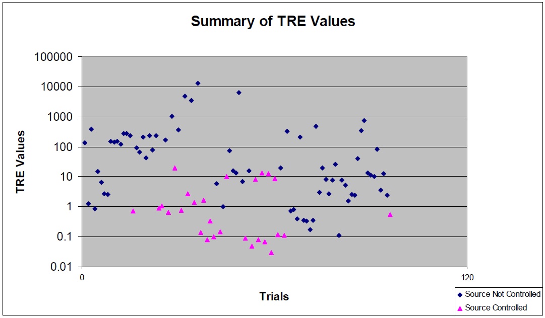
1.10 Discussion of TRE Results
TRE calculations result in values consistent with expectations. The TRE calculation methodology consistently results in values that are low for relatively high contaminant concentration sources and correspondingly higher TRE values for lower concentration sources. Recall that lower TRE values indicate more effective use of resources than higher values.
Importantly, the TRE methodology is validated through evaluations utilizing ‘reverse’ engineering. Sources that are currently operating with existing emission controls were evaluated as if the controls were not in place and consistently resulted in low TRE values. The conclusion is that the various engineering, business and regulatory processes that resulted in sources being identified for control in the past may be consistently predicted by the TRE methodology. This result should provide confidence that the TRE methodology can reliably indicate sources where it is appropriate to consider reduction action while providing structure, form, transparency and predictability to the process.
The dimensionless TRE value resulting from the methodology blends cost effectiveness and site specific risk reduction in a way that allows consistency of evaluation between sources and facilities. TRE values less than 1.0 fall within a range of acceptability recognized by industry and the Ministry based upon the results obtained from the ‘reverse’ engineered values shown in the table above. Further, TRE values ranging up to about 10.0 appear to represent a region where other factors need to be considered in determining the appropriateness of the reduction measure. TRE values much above 10.0 clearly fall outside the range of acceptability and represent relatively poor allocation of resources.
The risk score utilized in the TRE methodology effectively moderates cost effectiveness to reflect the ‘gravity’ of exposure to the contaminant being evaluated. Effectively, the magnitude of the site’s exceedence of the MOE standard increases the level of expenditure that may be appropriate (i.e. more resources should be expended by a site for greater eceedences of the standard). The frequency with which the standard is exceeded is used to moderate magnitude (i.e. the ‘gravity’ of the exceedence is reduced as the frequency decreases). The consequence of exposure to a contaminant is another factor considered in the risk score.
The consequence of exposure is derived from relative health effects scaling contained in GIASO. Major health effect contaminants are estimated to be 43% ‘worse’ than medium health effect contaminants and minor health and environmental effect contaminants are estimated to be 14% ‘better’ than medium health effect contaminants. These distinctions are relatively arbitrary and may not represent appropriate separation.
Calculations for sources emitting both TSP (medium health effect contaminant) and lead (major health effect contaminant) consistently indicated TRE values for lead control at least two orders of magnitude higher than TSP.
The data suggests that further evaluation is required to better determine the appropriate consequence distinction between major, medium and minor health contaminants. If POI reduction decisions are to be made based upon major health effects, then major health effect contaminants may have to be scaled at least 100 times greater than medium health effect contaminants. Another option might be to use surrogate contaminants for making POI reduction decisions (similar to the USEPA practice of using surrogate contaminants to evaluate HAP emissions). These are policy decisions that may require cross-functional stakeholder input (i.e. Ministry, industry, health, toxicology, and community representatives) and these data, unfortunately, do not inform that decision process.
1.11 Strength and Weaknesses of TRE Methodology
The following points describe some of the strengths and weaknesses of the Total Resource Effectiveness methodology and indicator in assessing a potential POI reduction technique’s cost effectiveness. Trials of the methodology have demonstrated the methodology to be robust and reliable. Further, the indicator value reliably identifies a threshold level for decision regarding the viability of POI reduction options. Retroactive application of the methodology to previously made decisions regarding installation of emission controls ‘ground truths’ the methodology and no inconsistent conclusions result.
1.11.1 Strengths
- Site specific and POI driven
- Considers potential risk of exposure in assessing appropriateness of potential reduction technique
- Relatively simple calculation to perform as part of an alteration of standard request
- Open and transparent evaluation
1.11.2 Weaknesses
- Consequence of exposure scale may not fully capture the spread of deleterious effects between contaminants
- Not a ‘bright-line’ test of potential POI reduction technique’s acceptability
- May result in different costs required for facilities within an industrial sector and between sectors
Appendix 1: Jurisdictional Review
2.1 Economic Indicators Used in Other Jurisdictions
This section of the report will present findings of how cost effectiveness indicators are used in other jurisdictions to evaluate control measure reasonableness and appropriateness.
Jurisdictions for review were selected based upon comparative relevance to Ontario in the following two parameters:
- Jurisdictions with an established manufacturing base comparable to Ontario.
- Established environmental regulatory systems to control air emissions.
State data regarding manufacturing sector, employment and capital investment was obtained from U.S. Department of Labor Bureau of Labor Statistics, US Census Bureau. US States comparable to Ontario in terms of manufacturing base, geographic location and environmental regulatory systems were selected for this report. Professional experience was used to select Countries comparable to Ontario in manufacturing capability and environmental regulatory structure. Following is a list of jurisdictions selected for review with a short rationale for each selection:
- US Environmental Protection Agency (USEPA) – A US cabinet-level federal regulatory agency that leads the nation’s environmental science, research, education and assessment efforts. It is charged with setting policy and guidelines, and carrying out legal mandates protecting the environment and the health and safety of people. USEPA coordinates all federal laws relating to the environment and enforces federal rules and requirements regarding environmental quality on federal agencies, state and local governments, and private individuals and firms. It is a long standing, most developed and highest resourced environmental agency in the world. Most of the original research in terms of environmental protection, including standards, controls and costs has been conducted by the USEPA.
- Michigan - A Great Lakes Basin State that borders Ontario on the South and shares its watershed and air shed. It ranks in the top 5 among the US States in terms of manufacturing capability, per data re: manufacturing entities, employment and capital investment. In addition to being a regional partner with Ontario it has a well established environmental regulatory structure that is comparable to Ontario.
- New York - A Great Lakes Basin State that is a regional partner with Ontario and shares a border, watershed and air shed. Its environmental regulatory regime is comparable to Ontario.
- Ohio – A Great Lakes Basin State and regional partner with Ontario. It ranks in the top five in US States in terms of manufacturing capability, per data re: manufacturing entities, employment and capital investment and has an environmental regulatory structure that is comparable to Ontario.
- Pennsylvania - A Great Lakes Basin State and regional partner with Ontario, with a comparable environmental regulatory system to control air emissions.
- Indiana - A Great Lakes Basin State that is a regional partner with Ontario. Its environmental regulatory regime is comparable to Ontario.
- Illinois - A Great Lakes Basin State and regional partner with Ontario. It ranks in the top five in US States in terms of manufacturing capability, per data re: manufacturing entities, employment and capital investment and has an environmental regulatory structure that is comparable to Ontario.
- Wisconsin - A Great Lakes Basin State and regional partner with Ontario, with a comparable environmental regulatory system to control air emissions.
- Minnesota - A Great Lakes Basin State that is a regional partner with Ontario. Its environmental regulatory regime is comparable to Ontario.
- California – Acknowledged as one of the most stringent regulatory systems for air pollution control and ranks in the top five in US States in terms of manufacturing capability, per data re: manufacturing entities, employment and capital investment.
- Texas - Ranks in the top five in US States in terms of manufacturing capability per data re: manufacturing entities, employment and capital investment.
- European Union (EU) – It is a political and economic community, established in 1993 of twenty-seven member states, located primarily in Europe. In 1996, the European Council, the highest political body of EU established the Integrated Pollution Prevention Control (IPPC) Directive, a high level regulation with a set of common rules for permitting, minimizing and controlling pollution from industrial installations, which is comparable to environmental regulations in Ontario. Europe has a diverse industrial base with manufacturing capabilities comparable to Ontario.
- United Kingdom – It has a broad and viable manufacturing base and an established environmental regulatory structure. It is a member of EU.
- Germany – Like the U.K., it is a member of EU with a broad and viable manufacturing base and an established environmental regulatory structure.
- Australia – It has an environmental regulatory regime and a manufacturing base comparable to Ontario.
2.2 Narrative Description of Cost effectiveness Indicators for each Jurisdiction
2.2.1 USEPA
Cost plays an important role in many State and Federal air pollution control regulations in the United States. The extent of this role varies with the type of regulation. Regulations such as Maximum Achievable Control Technology (MACT) standards explicitly use costs in determining their stringency. This has variously involved a balancing of costs and environmental impacts, costs and dollar valuation of benefits, or environmental impacts and economic consequences of control costs. Most often costs are calculated as the annualized capital and maintenance costs of air pollution control technology and the environmental impact is represented by the quantity of pollutants removed as a result of the application of control technology. This equation is expressed as $/ton, the numerator indicates the annualized cost of control and the denominator indicates the amount of pollutants removed. Some details regarding cost indicators used in several MACT standards will be presented later in this chapter.
The Best Available Control Technology (BACT) regulation also routinely employs cost effectiveness analysis in selecting the most appropriate and reasonable control technology for a given facility. Facilities applying for an air permit are required to demonstrate compliance with BACT by conducting a top-down analysis. Available technologies are identified, technically in feasible technologies are dismissed and the technically feasible technologies are ranked in terms of their effectiveness in pollutant removal. Once ranking has been completed, the facility than conducts a cost effectiveness analysis of the ranked technologies. (Cost effectiveness analysis is not required if the top ranked technology is selected). A $/ton value (calculated as shown above) is determined. Based on the $/ton value, if a technology is deemed to be prohibitively expensive then the facility is not required to employ it. They can move down to another technology with a lower ranking and so on down the list of ranked technologies. The short coming of this process is that the “prohibitively expensive” value is not defined. It is left to the regulating authority and the regulated facility to negotiate. Over the years however, a “rule of thumb value” has emerged that is applied fairly uniformly across the board.
Other types of regulations such as the National Ambient Air Quality Standards (NAAQS) use cost analysis to choose among alternative regulations with the same level of stringency. For these regulations an environmental goal is established by some set of criteria which do not include cost and then regulators use cost-effectiveness analysis to determine the minimum cost way of achieving the goal.
For some regulations, cost influences enforcement procedures or requirements for demonstration of progress towards compliance with an air quality Standard. For example, the size of any monetary penalty assessed for non-compliance as part of an enforcement action includes the cots of controls that were not installed by the noncompliant facility. Costs also play a vital role in EPA’s standard setting and regulatory development processes. Through various Executive Orders and Acts, USEPA has been charged with performing a number of detailed economic and benefit-cost analyses on each proposed rulemaking to assess their economic efficiency and assure the public that the best possible regulation has been chosen from among alternative regulations. The Office of Management and Budget (OMB) is required to review this analysis and either approve or disapprove the proposed regulation based on its economic efficacy. Additionally cost is considered in determining the economic impact of each regulatory alternative on sensitive populations, small business, employment, prices, market and industry structure.
In a vast majority of cases costs of air pollution control technologies are calculated using EPA’s Office of Air Quality Planning and Standards (OAQPS) manual. This manual provides cost data including capital costs, operating and maintenance expenses and other costs for air pollution control devices to industry and regulating authorities. In addition the OAQPS manual has established a standardized and peer reviewed costing methodology by which all air pollution control cost analyses can be performed. The manual has compiled up-to-date information on point and stationery area source air pollution control systems for Volatile Organic Carbons (VOCs), particulate Matter (PM), Oxides of Nitrogen (NOX), some acid gases (SO2 and HCl)for the past twenty five years. It should be noted, however that the data provide by the manual is nominally accurate to within ± 30%. Despite this shortcoming, the manual provides value. Industries can input their site-specific cost information into the standardized costing methodology provided by the manual to increase the accuracy of their cost effectiveness analyses. The advantage of using the standardized methodology is that it is recognized by both the regulating authorities and the regulated parties. When used in a permitting setting, the standardized methodology minimizes permit review time. Differences in conclusions are reduced to a comparison of input parameters, rather than a protracted debate on the veracity of alternative models. Additionally, the manual levels the playing field between the regulated entities by standardizing common assumptions such as the amortization period, interest rate etc.
On July 16, 1997, the President of the United States of America published a memorandum for the Administrator of the EPA, approving the issuance of revised air quality standards for Ozone and Particulate Matter (PM). The memorandum directed EPA to implement the new standards in a common sense, cost-effective manner. Towards that end, the memorandum declared $10,000 per ton of emission reduction as the high end of the range of reasonable cost to impose on sources. This action was expected to drive the development of new technologies with the potential of greater emission reduction at less cost (Presidential Documents, Federal Register, Vol.62, No.138, Friday July 18, 1997.
On July 24, 1997, EPA acknowledged that the States had the ultimate responsibility to attain the Ozone and PM standards and encouraged the Sates to design strategies for attaining these standards that focus on getting low cost reductions and limiting the cost of control to under $10,000 per ton for all sources. Additionally EPA pointed out that market based strategies could be used to reduce compliance costs. EPA encouraged the use of concepts such as Clean Air Investment Fund, which allow sources facing control costs higher than $10,000 a ton for any of these pollutants to pay a set annual amount per ton to fund cost-effective emissions reductions from non-traditional and small sources. Compliance strategies like these, EPA stated would likely lower the costs of attaining the standards through more efficient allocation, minimize the regulatory burden for small and large pollution sources, and serve to stimulate technology innovation as well (Mary Nichols, Assistant Administrator for Air and Radiation, EPA, Ozone and PM Standards, July 24, 1997).
Hazardous Air Pollutant (HAPs) emissions are regulated by the MACT standards. Following is a brief description of the MACT rules, which will facilitate the cost-effectiveness discussion of the various MACT standards, presented later in this section.
The 1990 Clean Air Act (CAA) Amendments established a new and fairly complex program to regulate emissions of HAPs (specific list of 187 chemical substances) from particular industrial sources. The Act required the USEPA to regulate emissions of these HAPs by developing and promulgating technology-based standards based on the best-performing similar facilities in operation. The national emission standards for hazardous air pollutants (NESHAPs) established by USEPA are commonly called MACT standards. MACT standards are designed to reduce HAP emissions to a maximum achievable degree, taking into consideration the cost of reductions and other factors. After the EPA adopts a MACT standard at the federal level, the State agencies propose the same standard for adoption at the state level.
When developing a MACT standard for a particular source category, the EPA looks at the current level of emissions achieved by best-performing similar sources through clean processes, control devices, work practices, or other methods. These emissions levels set a baseline, often referred to as the “MACT floor” for the new standard. At a minimum, a MACT standard must achieve, throughout the industry, a level of emissions control that is at least equivalent to the MACT floor. The EPA can establish a more stringent standard when it makes economic, environmental, and public health sense to do so.
The MACT floor differs for existing sources and new sources.
- For existing sources, the MACT floor must equal the average current emissions limitations achieved by the best-performing 12 percent of sources in the source category, if there are 30 or more existing sources. If there are fewer than 30 existing sources, the MACT floor must equal the average current emissions limitation achieved by the best-performing five sources in the category.
- For new sources, the MACT floor must equal the current level of emissions control achieved by the best-controlled similar source.
Wherever feasible, the EPA writes the final MACT standard as an emissions limit, a percent reduction in emissions or a concentration limit that regulated sources must achieve. Emissions limits provide flexibility for industries to determine the most effective ways to comply with the standards.
Sources subject to MACT standards are classified as either major sources or area sources.
- Major sources are sources that emit 10 tons per year of any of the listed HAPs, or 25 tons per year of a mixture of HAPs. These sources may release HAPs from equipment leaks, when materials are transferred from one location to another, or during discharge through emission stacks or vents.
- Area sources consist of smaller-size facilities that release lesser quantities of HAPs into the air. Area sources are sources that emit less than 10 tons per year of a single HAP, or less than 25 tons per year of a combination of HAPs. Though emissions from individual area sources are often relatively small, collectively their emissions can be of concern, particularly where large numbers of sources are located in heavily populated areas.
EPA has promulgated (or proposed) MACT Standards for 174 (major source and area) source categories.
The 2006 Proposed MACT rule for the synthetic organic chemical manufacturing industry, also referred to as the Hazardous Organic NESHAP (HON) rule discusses the cost-effectiveness of various control options in some detail. Cost was the determining factor in selecting regulatory control options. The five kinds of HAP emission points that are currently regulate by the HON are storage vessels, process vents, wastewater collection and treatment operations, transfer operations, and equipment leaks. The proposed rule considered two options for revising the HON rule. The first option (1) was to retain the current rule and the second option (2) was to require more stringent standards for the emission points. The current HON control requirements for process vents cost $3000 per ton of HAP removed. The additional controls proposed were estimated to cost $15,000 per ton removed. This cost was considered unreasonable. The estimated cost of installing additional control on storage vessels (internal floating roofs on existing fixed roofs) was $12000 per ton of HAP removed. This was considered reasonable and included some caveats to ensure the cost did not exceed $12,000 per ton. The estimate to develop additional control measures for process wastewater streams was greater than $12,000 per ton, which was concluded to be unreasonable. For leaking valves, several additional options were considered. The option considered reasonable had a cost-effectiveness number of $11,000 per ton. Further controls on transfer operations were estimated to cost between $10,000 per ton to $100,000 per ton. These costs were considered unacceptable and it was concluded that transfer operations did not require further controls. In the final analysis of the entire source category, EPA estimated that the additional costs of further control, as represented by option 2, were an average of $8,000 per ton HAP removed and an incremental cost of $10,000 per ton of HAP removed. EPA concluded that the additional costs of further controls (option 2) when compared against the relatively small reductions in health risks achieved by that alternative, called for no changes to the current HON rule, i.e. no further controls (Proposed HON NESHAP, Federal Register, Vol.71, No.114, Wednesday June 14, 2006).
2.2.2 Michigan
The Air Quality Division (AQD) of the Michigan Department of Environmental Quality (MDEQ), under its delegated authority from USEPA has developed and operates various air permitting programs. A BACT analysis (top down analysis) is one of the corner stones of the programs and is employed during the permitting process to determine the controls required for criteria pollutants, especially VOC, at the facility applying for the air permit. The AQD has published a memorandum that provides guidance on performing the BACT analysis. Although cost effectiveness is one of the factors considered in the selection of the control equipment at a given facility, a specific threshold value of economic acceptability is not published. Rather, it provides direction that energy, environmental, and economic impacts can be considered.
The memorandum further states that evaluations of energy or environmental impacts are generally assessments of unusual impacts at the facility under review compared to impacts at other recently permitted facilities. The consideration of these collateral impacts is used to either confirm the top BACT option as appropriate or to demonstrate that it is inappropriate. Impacts, such as costs (i.e., dollars per ton of pollutant removed), borne by recently permitted similar facilities is the standard used to determine whether an impact is economically appropriate. In essence, it comes down to a case-by-case determination made by the AQD permit Engineer, guided by engineering principles and agency experience concerning practicality and impacts of an emission reduction option, of whether the facility satisfies the BACT requirements (Michigan Department of Environmental Quality, Air Quality Division, Operational Memorandum No. 20, BACT Determinations, August 24, 2005).
2.2.3 California
The federal government, primarily through the EPA, sets standards, oversees state and local actions, and implements programs for toxic air pollutants, heavy-duty trucks, locomotives, ships, aircraft, off-road diesel equipment, and some types of industrial equipment. State government, through the Air Resources Board and Bureau of Automotive Repair, sets more stringent state standards, oversees local actions, and implements programs for motor vehicle emissions, fuels, and smog checks. Local air pollution control districts, such as the San Joaquin Valley Air Pollution Control District (Valley Air District), develop plans and implement control measures in their areas. They issue air permits to stationery sources and hence implement BACT regulations.
The San Joaquin Valley, Air Pollution Control District which is made up of eight counties in California’s Central Valley published a BACT policy in 1999, to ensure that BACT determinations were made in a timely and uniform manner. The policy provides step-by-step guidance on the BACT top-down analysis. Additionally it provides guidance on performing a cost-effectiveness analysis. The analysis is similar to the one described in the OAQPS manual.
However, the San Joaquin District goes further and declares a cost-effectiveness threshold for criteria pollutants. The table is reproduced below (Table 1).
| Pollutant | Cost Effective Threshold (US$/ton) |
|---|---|
| VOC | 5000 |
| NOX | 9,700 |
| PM10 | 5,700 |
| SOX | 3,900 |
| CO | 300 |
The policy states that a control technology, including control equipment or alternate process, whose cost has been calculated according to the guidance provided in the Policy, reveals that the annual cost per ton of controlling each affected air pollutant is less than the Cost Effective Threshold(s) specified in the above Table, is required a cost effective control. Controls that are not cost effective shall be eliminated from consideration (unless the control is achieved in practice or required by an EPA approved SIP). The policy further defines a Multi Pollutant Cost Effectiveness Threshold (MCET) with an illustrative example reproduced below:
Example: If a control strategy reduces 2 tons of NOx, 4 tons of SOx, and 0.1 ton of particulate matter, the MCET would be calculated as follows:
MCET = (2 tons NOx/yr) × ($9700/ton NOx) + (4 tons SOx/yr) × ($3900/ton SOx) + (0.1 ton PM/yr) × ($5700/ton PM) = $35,570 per year
If the total annual cost, (Step 3) exceeds this MCET, the control technology or equipment under review can not be required as BACT. If a control technology or equipment is not cost effective, the cost effectiveness analysis for the next less stringent control technology or equipment is performed as appropriate (San Joaquin Valley Unified Air Pollution Control District BACT Policy, November 9, 1999).
2.2.4 Ohio
Ohio Administrative Code (OAC) rule 3745-31- 03(A)(3) of the Ohio Environmental Protection Agency (OEPA) requires, that any person intending to install a new source - or modify an existing source - of air emissions apply for and obtain a permit-to-install (PTI). The PTI requires a Best Available Technology (BAT) analysis. BAT is defined in Ohio Revised Code (ORC) section 3704.01(F) and OAC rule 3745-31-01(N) as: Best Available Technology is any combination of work practices, raw material specifications, throughput limitations, source design characteristics, an evaluation of the annualized cost per ton of air pollutant removed, and air pollution control devices that have been previously demonstrated to the director of environmental protection to operate satisfactorily in this state or other states with similar air quality on substantially similar air pollution sources.
The review of PTI applications is conducted by local air agencies and OEPA district offices. OEPA considers cost analyses an important aspect of the review. To ensure that the costs are derived in a consistent manner and to promote statewide uniformity, OEPA published engineering guide No. 46 to provide guidance on cost estimating and related methodologies, for estimating costs for air pollution control systems. This guide outlines the process for estimating capital costs, annual operating costs and the annualized cost of a pollution control device or control measure. The guide discusses cost-effectiveness expressed as the annualized cost ($) per ton of emissions reduction achieved by the control. This guide does not provide any information related to whether a particular cost-effectiveness value ($/ton of emissions reduction) is representative of BAT. The methods and procedures presented should provide cost estimates accurate to within ±20 to 30 percent for specific cases where adequate data are available. The guide clearly states that the determination of whether or not a particular cost effectiveness value is economically reasonable is not within its scope. The Agency in other communications, such as response to comments, states that economic appropriateness will be made on a case by case basis.
2.2.5 All Other US States Reviewed
Other state programs reviewed for this report include, Pennsylvania, New York, Wisconsin, Minnesota and Texas. All States had permitting processes that were a slight variation of the Ohio and Michigan programs. All of them required BACT or BAT analysis (similar), including a cost effectiveness analysis component. Although cost was a consideration in the overall requirement of BACT or BAT demonstration, a value has not been declared. It is usually a case by case determination, guided by technologies or practices for limiting emissions that have been proven for a similar operation. For example, if a review finds that many existing operations of the same type are employing a raw material, work practice or “add-on” control that limits emissions, then it is likely that BACT or BAT will be considered to be similar. In some cases, an applicant may demonstrate a new or modified operation will employ superior emission control to every other operation in its industry. With suitable documentation, the new or modified operation could be approved. Last but not the least, a rule of thumb value has emerged over the years, it is $6000 - $8000. Typically control technologies with a cost effectiveness value of greater than 8000$/ton are not required.
2.2.5 European Union
The European Council through Directive 96/61/EC, established the Integrated Pollution Prevention and Control (IPPC) rules. The IPPC regulations employ an integrated approach to control the environmental impacts of certain industrial activities/sectors. It involves determining the appropriate controls for industry to protect the environment through a single permitting process.
Article 16(2) of the IPPC Directive requires the European commission to organize and exchange information between member states and between member States and the industries concerned on best available techniques, associated monitoring and developments in them”, and to publish the results of the exchange. The Commission published the results as the BAT Reference documents (BREF notes) for each of the 30 sectors. The BREF notes do not constitute binding requirements, but regulatory authorities in the member states are encouraged to take them into account in their own determinations of BAT. The IPPC requires the operators to choose the best option available to achieve a high level of protection of the environment taken as a whole. Operators are required to demonstrate best available techniques (BAT). This, together with a consideration of local circumstances, and economics provides the main basis for setting Emission Limit Values. BREF notes provide guidance to both regulators and operators on BAT requirements. While they encourage a cost effective approach, provide guidance on calculating costs (both capital as well as annual), they do no provide specific cost effectiveness values, or monetary values or thresholds that can be used to determine economic appropriateness or reasonableness.
2.2.6 U.K.
The IPPC Directive was enacted into English law through the Pollution Prevention and Control (England and Wales) Regulations on 1st August 2000 and implements the EC Directive 96/61/EC on IPPC. In essence, IPPC legislation increases the scope of coverage of existing Integrated Pollution Control (IPC) legislation, introducing a number of new industry sectors, and extends the topic base of items that require attention by the operator of an installation. Separate Regulations apply the IPPC Directive in Scotland and Northern Ireland and to the offshore oil and gas industries.
The permit application requires the operator of an installation (facility) to prepare a forward plan to deliver the elements of IPPC, at a suitable cost and in a timely fashion. It includes:
- Demonstrating a satisfactory Environmental Management System (EMS), including critical control systems and procedures
- Justification of Best Available Techniques (BAT) at the installation, using site specific criteria and cost benefit analysis.
- A full understanding of pollutant releases from the installations and environmental impact assessments of the releases (for example, chemical pollutants, noise etc).
- A site condition report.
- Energy, water & waste minimization audits and recommendations.
- A raw materials conservation study.
Domestic guidance was produced on required standards and Best Available techniques (BAT) for the individual sectors, drawing on the information contained within BREF notes. This guidance contains clear, indicative standards for both new and existing installations. It also contains timetables for upgrading existing installations.
The Department for Environment Food and Rural Affairs (DEFRA) published a practical guide on the IPPC in June 2005. Cost effectiveness of air pollution control is addressed in the BAT section of the guide. The guide states that the BAT approach ensures that the cost of applying techniques is not excessive in relation to the environmental protection they provide. It explains that the more environmental damage BAT can prevent, the more the regulator can justify telling the operator to spend on it before the costs are considered excessive. The process is similar to the US BACT in that once the options are ranked, the option that minimizes environmental impact from the installation will be BAT unless economic considerations renders it unavailable. The cost assessment is required to include operating costs as well as capital costs. This should include any cost savings.
The guide (as the BREF notes) does not specify a cost threshold or a Cost/pollutant removed value above which a control option is not considered viable. It provides narrative guidance as follows:
An objective approach needs to taken to balancing costs and advantages when assessing what are BAT. The lack of profitability of a particular business should not affect their determination. For example, if it has been established that a particular technique is BAT within a certain sector, then the regulator should normally impose the ELVs (Emission Limit Values) that correspond to the use of that technique in all permits for that sector. However, there may be some cases where the regulator should set different standards, for example because the balance of costs and benefits is different in the particular local environmental and/or technical circumstances of a particular installation. But it would not be right to authorize lower standards, or to delay the implementation of BAT solely because an operator argued for this narrowly on the basis of its own financial position. Conversely, the regulator should not impose stricter standards than BAT just because an operator can afford to pay more.
(The Department for Environment Food and Rural Affairs, IPPC, Practical Guide, June 2005).
2.2.7 Australia
Protection of the Environment Operations (Clean Air) Regulation 2002, Part 4, Emission of air impurities from activities and plant is the enabling regulation to control air pollution from industrial sources. The regulation makes no mention of cost or cost effectiveness. (NSW Legislation)
2.2.8 Germany
As required by Directive 96/61/EC, Germany has adopted the IPPC and the associated BREF notes. In addition, the German Federal Environment Agency (Umweltbundesamt - UBA) is in the process of consolidating all environmental laws governing different sectors and applying to different media into one comprehensive environmental code (Umweltgesetzbuch - UGB). It is not certain how cost effectiveness will be addressed in the environmental code. Traditionally, the German Federal Environment Agency has not considered cost benefit analysis. As per Dr. Axel Friedrich Umweltbundesamt (UBA), Germany, December 2004, in Germany the cost benefit approach is not used because they do not believe that costs or benefits can be accurately determined. (Dr. Axel Friedrich Umweltbundesamt (UBA), Germany, Cost effectiveness of AQM in Germany, December 2004). However, as required by the Directive 96/61/EC, Germany has adopted the IPPC and the associated BREF notes. Although BREF notes do no provide specific cost effectiveness values, or monetary values or thresholds that can be used to determine economic appropriateness or reasonableness, they encourage a cost effective approach and provide guidance on calculating costs (both capital as well as annual). It is expected that the German environmental code will adopt the same approach.
Attachments
Example Forms
Figure 3: POI Reduction Technique
Blank Forms
TRE Calculations for Thermal Oxidizers
TRE Calculations for Venturi Scrubbers
Footnotes
- footnote[1] Back to paragraph See GIASO for a definition of the Net Total Annualized Costs (NTAC).