An Algal Bioassessment Protocol for use in Ontario Rivers
The Algal Bioassessment Protocol (ABP) was designed to complement other water monitoring programs already in place in Ontario, such as the Provincial Water Quality Monitoring Network, the Ontario Stream Assessment Protocol and the Ontario Benthos Biomonitoring Network.
Prepared by:
Ontario Ministry of the Environment
Environmental Monitoring and Reporting Branch
Toronto and Region Conservation Authority
Last Revision Date: December 2011
Cette publication hautement spécialisée n’est disponible qu’en anglais en vertu du règlement 441/97, qui en exempte l’application de la Loi sur les services en français. Pour obtenir de l’aide en français, veuillez communiquer avec le ministère de l’Environnement au
For more information:
Ministry of the Environment
Public Information Centre
Email: picemail.moe@ontario.ca
Website: Ministry of the Environment and Climate Change
PIBS 8618e
Executive Summary
The Algal Bioassessment Protocol (ABP) was designed to complement other water monitoring programs already in place in Ontario, such as the Provincial Water Quality Monitoring Network, the Ontario Stream Assessment Protocol and the Ontario Benthos Biomonitoring Network.
Comprehensive water monitoring programs incorporating physical, chemical and biological monitoring, including benthic algae, have been successfully implemented in New Zealand, the U.S.A. and many of the European Union countries. The need to monitor not only the physical and chemical changes in the aquatic systems, but also the biotic response to change, has been recognized and implemented in these national water monitoring frameworks.
The addition of algal monitoring to water chemistry and benthic invertebrate monitoring programs permits an integrated assessment of water quality. Responses to changes in water quality occur over different time scales for primary producers and consumers, as primary producers often respond to changes earlier. By integrating the ABP with water chemistry and benthic invertebrate monitoring, an evaluation of both the physical and chemical changes as well as the resulting biological responses becomes possible. This method of monitoring provides an early warning system of changes in the health of our aquatic ecosystems.
Background
Introduction to benthic algae
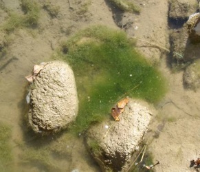
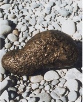
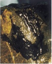
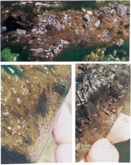
Periphyton, or benthic algae, play an important ecological role in all aquatic environments. Recognizable as films or filaments covering rocks or other substrates in rivers and along the shorelines of lakes, periphyton serve as a link between the physico-chemical environment and the biota. Like plants on land, periphyton photosynthesize; they acquire nutrients from the surrounding water and turn them into useful organic molecules and energy. Due to this direct reliance on the water, benthic algae are particularly sensitive to water quality changes and the composition of the algal community will change in response to changes in water quality.
Figure 1: Green algal figments growing on rocks
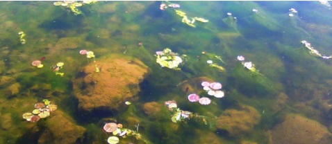
The sensitivity of algae to changes in water quality is key to their use as indicators of physico-chemical conditions in aquatic ecosystems. When contamination occurs, algae are among the first biological organisms to respond. This is a result of their short lifespan, which averages about 6 to 8 weeks. Additionally, algae are generally immobile and unable to move away from contamination. Those species that cannot tolerate the water quality changes will be replaced by species better suited to the new water quality conditions, resulting in an altered algal community composition. Consequently, the composition of a diatom community is a reflection of water quality conditions over the previous 1 to 2 months (Taylor 2004; Walsh and Wepener 2009).
Because algae are sensitive to changes in water quality and have a short life span, they are ideal indicators of environmental change. They respond strongly and predictably to changes in water quality and are easily sampled and identified. As a result benthic algae have a long history of use in water quality monitoring.
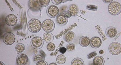
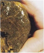
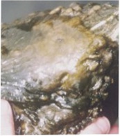
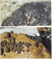
Diatoms are an important component of the periphyton community and are especially suitable as biological indicators of water quality. Diatoms are microscopic algae represented by over 100,000 species worldwide and can be recognized in rivers and from the shoreline areas of lakes as the brown, slippery coating on submerged substrates like sand or rocks. There are a number of advantages to using diatoms as biological indicators as compared to other algal groups. Diatoms have cell walls (frustules) with species-specific features, making them readily identifiable under a microscope. Their taxonomy is well known and well described, as are the environmental optima and tolerances of different species. Because their cell walls are made of silica, which resists degradation, historical water quality conditions can be estimated using diatom frustules preserved in sediment from lake bottoms and stable areas of streams and rivers. Recently some researchers have also recovered diatoms from the stomach contents of fish archived at the Royal Ontario Museum. They analyzed the preserved populations from several Ontario streams to compare the diatom communities from the 1920s and 1930s to present-day communities to assess changes in water quality (Lavoie and Campeau 2010).
Relationships with water chemistry
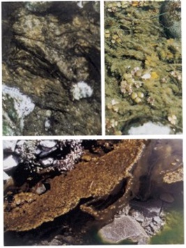
The structure of algal communities is strongly influenced by water chemistry. Algal growth and taxonomic composition respond predictably and sensitively to nutrient enrichment, organic contamination, changes in pH or conductivity as well as increases in suspended sediments, pesticides and many other contaminants. Many studies have recognized the strong link between nutrient availability and diatom community structure, and have attributed a large percentage of the community variation directly to the nutrients present (Dodds et al. 2002; Hill 2003; Blanco and Becares 2010; Torrisi et al. 2010). Others have found strong correlations between pH, dissolved oxygen, alkalinity, conductivity and substratum conditions and the structure of the diatom community (Blinn and Herbst 2003). A study conducted in southern Quebec and eastern Ontario identified that electrical conductivity was the most influential water quality variable impacting diatom communities (Zugic-Drakulic 2006). High concentrations of heavy metals can also impact the diatom community, causing frustule deformities and loss of diversity (Walsh and Wepener 2009; Duong et al. 2010).
Figure 2: Microscope view (400× magnification) of diatoms from Lake Simcoe
Water chemistry sampling provides information on the concentration of chemical parameters at the instant a sample was collected; results do not necessarily indicate conditions in the days or even minutes before sampling. Consequently, routine chemical monitoring programs can miss short-term changes in water quality, such as storm run-off or environmental spills whereas biological communities continuously respond to changes in water quality. Sudden changes in water quality, like storm run-off, along with more long-term or gradual changes result in shifts in the composition of the diatom community. This results in a community whose composition reflects the water quality conditions it has been exposed to over the previous 1 to 2 months (Taylor 2004; Lavoie et al. 2008; Walsh and Wepener 2009).
The benthic invertebrate community also responds to water quality changes, but its response is slower and may not be evident until 4 to 6 months later (Soininen and Kononen 2004). This response is due to the longer lifespan of benthic invertebrates as compared to diatoms. Additionally, the autotrophic diatom community has a direct dependency on the water to provide nutrients and minerals. Diatom communities are particularly responsive to chemical changes such as organic enrichment and contamination with pollutants or metals. The monitoring of benthic invertebrates together with benthic algae provides an integrated assessment of water quality and provides water managers with information about current water quality conditions, as well as an indication of how the water quality has changed over the previous six months.
Benthic algae for water quality monitoring
Studies using periphyton for biomonitoring were first published by Kolkwitz and Marsson in 1908 (cited by Hering et al. 2006). More recently, the specific advantages of using diatom assemblages for monitoring water quality have become recognized worldwide, with monitoring initiatives across Europe, the and South Africa. Several countries have recently developed successful, user-friendly and comprehensive monitoring protocols such as New Zealand’s Stream Periphyton Monitoring Protocol (Biggs and Kilroy 2000) and the U.S.’s Periphyton Protocol (Stevenson and Bahls 1999). In 2000, the European Union set the standard for aquatic monitoring by mandating that all European Union countries use various biological organisms (including diatoms) for monitoring stream health as part of the Water Framework Directive (Hering et al. 2006; Stoddard et al. 2006).
The use of benthic algae in bioassessments within Canada has been inconsistent. Studies have mainly focused on nutrients. Winter and Duthie (2000) used diatom assemblages to predict nitrogen and phosphorus concentrations in representative southern Ontario streams with a gradient of urban and agricultural land uses. Nitrogen and phosphorus optima and tolerances for 66 of Ontario’s diatom species were determined as well. Others have used diatoms in eutrophication studies, either to differentiate nutrient loading from general organic pollution (Rott et al. 1998), or to determine threshold levels for total nitrogen and total phosphorus to protect ecosystem health (Chambers et al. 2008). However, reports using periphyton community composition to evaluate stream health have been rare and those that were completed often relied on algal indices developed overseas.
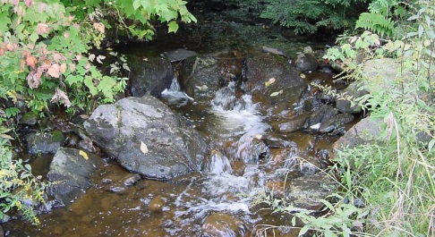
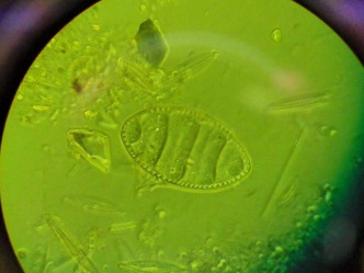
Figure 3: A stream in the Muskoka, Ontario area
The first Canadian broad-scale studies to use benthic algae as bioindicators of water quality were conducted in Quebec. Lavoie et al. (2004) evaluated the composition of the diatom community in relation to land use and water quality. The authors’ studies on streams in Quebec and several sites in Ontario identified a strong relationship between the composition of the community and the general state of water quality and resulted in the development of the first Eastern Canadian Diatom Index (IDEC). The IDEC compares the diatom community composition at one sampling location to the community composition that would be expected at the same location if it was unimpacted (Stoddard et al. 2006). It is a “chemistry-free index”; sites are positioned according to how similar their diatom community composition is to the expected reference community. Scores range from 0 to 100, with lower scores indicating more impaired or biologically atypical sites and higher scores indicating a diatom community that is less impacted. For more information on the IDEC, refer to Appendix 1.
The development of an algal bioassessment protocol in Ontario
Simultaneously, the Ontario Ministry of the Environment (MOE) began to develop a benthic algal monitoring protocol to complement its existing monitoring programs, such as the Ontario Benthos Biomonitoring Network and the Provincial Water Quality Monitoring Network. Studies to direct the development of a benthic algal monitoring protocol began in 2002 as a partnership between the Toronto and Region Conservation Authority (TRCA), the University of Toronto and the MOE. The project examined the community composition of diatom samples collected from different substrates (rocks, sand, macrophytes) and the applicability of a three-tiered assessment: (1) a rapid visual assessment, (2) a rapid identification under the microscope, and (3) a high resolution identification of diatoms to species level. Differences in the amount of time required for each method, as well as differences in the level of expertise and taxonomic precision required, were considered important to determine the most useful assessment level, both in terms of taxonomic detail and practicality.
The results of this initial study indicated that the third approach, high resolution taxonomic identification of the diatom community, showed the strongest and most useful relationship with water quality (Zugic-Drakulic 2006). This finding agrees with the conclusions of the work to develop the IDEC (Lavoie 2004), which also found that analysis using only diatoms was the optimal approach. The end result of this project was the development of a preliminary benthic algal monitoring protocol.
The second phase of the project was designed to determine if the variability between samples collected by different crews was significant. To do this, paired samples were collected by two independent crews from sites across the TRCA's jurisdiction (in 2008), and from across southern Ontario (in 2009). Analysis involved comparing the taxonomic composition of the samples collected by each of the two crews. The results of this study indicated that the protocol produced the repeatable and comparable results needed for an effective, standardized protocol (see Box 1).
Box 1. The need for a Standardized Monitoring Protocol
Biomonitoring in Ontario has traditionally been approached at a watershed or regional scale, with individual monitoring groups often developing programs on their own with little collaboration between agencies. As a result, data from different biomonitoring programs were often not comparable due to inconsistent methods and data management. By standardizing monitoring and analytical methods, and by creating common databases, data from individual groups becomes comparable across watersheds, allowing larger-scale reporting at the provincial and possibly national scale (Borisko et al, 2004). Examples of programs where such standardization has been achieved include the Ontario Benthos Biomonitoring Network (OBBN) and the Ontario Stream Assessment Protocol (OSAP). The algal bioassessment protocol (ABP) reflects methods already used in a variety of monitoring projects and provides another standardized indicator for evaluating water quality in Ontario rivers.
The Algal Bioassessment Protocol
The Algal Bioassessment Protocol (ABP) is designed to assess aquatic ecosystem conditions in wadeable streams using benthic algae as indicators of water quality conditions. The protocol describes three modules for the collection and visual assessment of diatoms and soft algae.
Module 1: Diatom Sample Collection
This module is strongly recommended as it describes the collection of diatom samples from hard and soft substrates within a monitoring site.
Module 2: Soft Algae Sample Collection
This module describes the collection of soft (filamentous) algae samples from substrates within a monitoring site. This module is undertaken in conjunction with Module 1 and is optional.
Module 3: Visual Assessment of Algae
This optional module describes a technique for visually describing the different types of algal communities present at a stream site. Visual assessments may be conducted either independently or to supplement other modules. Visual assessments are most applicable to first- and second-order streams and have proven useful for tracking changes in water quality in small streams when applied by the same crew between years or sites.
Module 1: Diatom Sample Collection
Introduction
This module describes the sampling technique for collecting diatom samples from hard and soft substrates within a site. Results from these surveys can be used in bioassessments or as indicators of water quality conditions.
Pre-Field Activities
Diatom sampling requires a crew of two people and collection time of about 10 - 15 minutes. Additional time is required for sample processing, slide preparation and taxonomic identification (see Appendices 1 and 2).
Pre-field activities should include:
- Obtaining landowner permission on private land
- Documentation of site access and site identification
- Equipment check
Equipment List
- 'Algae Collection Form' datasheets, on waterproof paper
- Waders
- Pencils
- Turkey baster
- Toothbrush
- Squirt bottle filled with tap water
- Sample bottles for diatoms (1 per site)
- Brush/syringe sampler
- Labels or permanent marker
- Scalpel, pocket knife or other sharp knife (e.g. small kitchen knife) in a protective carrier
- Small ruler
- Lugol’s preservative
- Small bottle of 10 % bleach solution
- A device for measuring water quality analytes (e.g. dissolved oxygen, pH, conductivity, dissolved organic carbon, etc.) is also recommended.
Crews should adhere to safety precautions and requirements set forth by their employers i.e. first aid kit, first aid and other training, chemical handling procedures, travel plan, buddy system, mobile phone, etc.
Site Selection
Diatom sampling is generally done in riffles; therefore your site should contain at least one riffle if possible. A riffle is an area of relatively fast, turbulent flow, where the water’s surface is typically broken and has an obvious slope (see Figure 5).
Figure 5: Stream reach illustrating areas of slow flow (pools), fast flows (riffles) and intermediate flows (runs) (adapted from Jones et al. 2007)
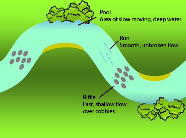
Riffle areas with hard substrates (gravel, cobble, boulders) are preferred. If you do not have any riffles in your sampling location, look for a run (an area with smooth, fast flow) preferably with stony substrates (rocks rather than sand or silt).
Algal surveys must not be conducted for at least 2-3 weeks after a bottom-scouring storm event. Bottom-scouring storm events are defined as heavy rain storms that produce floods or high flows and strong velocities capable of moving the substrate particles of the size that characterize the site. Such events disrupt algal communities attached to substrate particles. Samples collected soon after a scouring event will not represent ambient water quality. Therefore, you must delay sampling to allow time for re-colonization.
Recording Information about the Site
If algal sampling is not being conducted concurrently with either OSAP or OBBN sampling, then additional information about the site will need to be collected. At a minimum, record the site code, location (on a map or use UTM co-ordinates) and a sketch of the sampling site. The sketch should show direction of stream flow, indicate where the algal sample was collected, and show site boundaries (and markers if used). See S1.M1 Screening Level Site Documentation of the OSAP manual for more information (Stanfield 2010).
Locating the Collection Areas
Within your sampling site, choose 5 locations where you will collect samples. Locations receiving sunlight are preferred; if possible sample in areas receiving sunlight at midday. All five sampling locations do not need to be in the same riffle (see Figure 6).
Figure 6: Five sampling locations in one site (adapted from Jones et al. 2007)
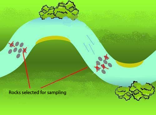
Diatoms will be collected from substrate particles selected from the tream bed. Only one type of substrate may be sampled at each site. The preferred substrate for diatom sampling is a rock; however, if there are no rocks in your site you may sample another substrate type from the list below. You must select the same substrate type for all 5 samples.
Order of substrate preference
- rocks, cobble, boulders
- woody debris
- fine sediments (sand, silt, clay)
- plants
Begin the survey at the collection area that is farthest downstream and move upstream as you sample to avoid disturbing downstream collection areas.
Collecting the Diatom Sample
- Before collecting the sample, label your diatom sample jar with the following information:
- Site code
- Date of sampling
- Substrate sampled
- Name of person collecting the sample
- Type of sample (diatom)
- Preservative used
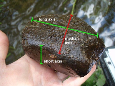
- Beginning at the downstream collection area, reach down and select a rock (or other preferred substrate). Make sure the substrate particle you select is completely submerged in the water. For removable substrates such as rocks, target those with a median axis of at least 40 mm (see Figure 7).
- Make a note of which side of the substrate was facing up, exposed to sunlight. This is the surface you will sample from.
- If you are opting to collect soft algae as well as diatoms please see Module 2: Soft Algae Sample Collection.
- If filamentous algae are present, measure the longest filament of algae to the nearest mm and record.
- Measure and record the median axis of the substrate particle. Every object has 3 dimensions: length, width and height. The median axis is the dimension that has the intermediate measurement. In Figure 7 the median axis is the red line.
Figure 7: Measuring the median axis
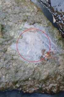
- Collect your diatom sample from the side of the particle that was exposed to sunlight using the methods described in Table 1. In order to collect enough material you must sample an area of at least 2500 mm2 (the size of a loonie at 28 mm diameter; see Figure 8).
- Move upstream to the next collection area and repeat steps 2 to 6. Continue to collect the diatom samples in the same jar, until you have collected from five collection areas.
Figure 8: Scraped area sampled on a rock
- After you have collected and pooled your five samples into one jar there should be between 50 and 150 mL of water in the jar. Preserve the sample by adding 1.0 mL of Lugol’s preservative solution. The water in the sample jar should now be a light tea colour. If it is not, add extra Lugol’s by drop until the water is a light tea colour.
- Examine all brushing and scraping tools for any residues. Before sampling the next site, thoroughly rub and rinse them clean in tap water, then wash with a 10 % bleach solution and give them a final rinse with tap water. Ensure all tools are washed as described and then dried before storage.
| Substrate type | Collection Method |
|---|---|
| Hard, removable substrates > 40 mm median axis (gravel, cobble, woody debris) |
|
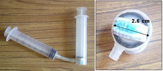
| Hard, large, non-removable substrates (that are submerged) (boulders, bedrock, logs) | Use a brush / syringe type of sampler. See Figure 9 below.
|
| Fine sediments (silt, mud, clay) |
|
| Fine sediments (sand) |
|
| Plant material (mosses, macroalgae, vascular plants) |
|
Preparing and Processing the Sample
Figure 9: Syringe sampler for submerged substrates (from Thomas and Hall 2009)
If you are planning to prepare and identify algae contained in the sample, follow steps in Appendices 3 and 4. Alternatively, you may have a diatom taxonomist identify the collected algae.
Module 2: Soft Algae Sample Collection
Introduction
Soft algae (for the purposes of the ABP), are defined as all types of algae except diatoms. The use of soft algae in biomonitoring requires different collection and preservation methods than those used for diatoms. Because proper identification of this group relies partially on colour, preservation using either Lugol’s solution (which is mainly iodine) is not effective. Samples can either be refrigerated and identified within 2 days or preserved in 10% formalin.
This optional module describes the collection of soft algae samples to supplement the diatom samples collected using Module 1.
Pre-Field Activities
The time required to collect soft algae is approximately 5 minutes.
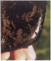
Figure 10: Filamentous algae
Equipment List
- ‘Algae Collection Form’ datasheets, on waterproof paper
- Waders
- Pencils
- Squirt bottle filled with tap water
- Sample bottles for soft algae (1 per site)
- Brush/syringe sampler
- Labels or permanent marker
- Scalpel, pocket knife or other sharp knife (e.g. small kitchen knife) in a protective case
- Small ruler
- 10% formalin preservative
Field Procedures
Diatom sampling (Module 1) is the recommended module of the ABP. If also collecting a soft algae sample it is recommended that you complete both modules together, following the field procedures in Module 1. You will use the same datasheet (Algae Collection Form) for the soft algae sample collection.
Note: Soft algae samples are collected at the same time as diatom samples. You will use the same substrate (if possible) and will need 2 loonie-sized collection areas.
Collecting the Soft Algae Sample
- Before collecting the sample, label your soft algae sample jar or bottle with the following information:
- Site code
- Date of sampling
- Substrate sampled
- Name of person collecting sample
- Type of sample (soft algae)
- Preservative used
Once you have selected your sample substrate and measured the longest filament, you can collect your soft algae sample.
- Select two areas on your substrate particle from which you will collect samples. Each area must be approximately the size of a loonie (28 mm diameter). Remember to select an area that has been exposed to sunlight.
- Using a knife, cut the filamentous algae off the substrate from one of these areas and place the cuttings in the soft algae sample jar.
- Scrape the same area and place scrapings in the soft algae sample jar (the same one as the filament cuttings).
- Rinse the knife with tap water, directing the rinse water into the soft algae sample jar.
- Using the second loonie-sized collection area on your substrate particle, collect the diatom sample following the methods in Module 1.
- Repeat sampling procedure (steps 2 to 6) at each of the 5 collection areas, pooling all the soft algae samples into one jar and all the diatom samples into a second jar.
- Preserve the soft algae sample with 10% formalin or refrigerate and identify soft algae within 2 days. Preserve the diatom sample according to the methods in Module 1.
Preparing and Processing the Sample
Soft algae samples can be homogenized by blending, although subsamples of large filamentous algae should be examined intact under a dissecting microscope. A drop of the homogenized sample can be mounted on a microscope slide and covered with a cover slip for counting. Methods for processing soft-algae samples and conducting relative abundance assessments or cell counts are outlined in Biggs and Kilroy (2000) and Lowe and LaLiberte (2007).
Module 3: Visual Assessment
Introduction
Visual assessments are conducted by observing the different types of algal communities present at a stream site. They are most useful in 1st- and 2nd-order streams. Follow-up visual assessments should be conducted by the same person or crew conducting initial assessments, as some of the factors (colour, texture, etc.) can be subjective. Visual assessments may be conducted either independently or in conjunction with either diatom and/or soft algae sample collection.
Pre-Field Activities
The time requirement to complete a visual assessment survey is 30 to 45 minutes.
Equipment List
- ‘Algae Visual Assessment’ datasheets, on waterproof paper
- Waders
- Metre measuring stick (wooden)
- Pencils
- Periphyton field identification chart
- Small ruler
- Tea strainer
- Digital camera
Setting up Transects
Within the sampling site establish 3 transects across the width of the stream, each with similar substrate, depth and flow characteristics. Riffle areas with hard substrates (gravel, cobble, boulders) are preferred. If you cannot establish 3 transects that are within riffle areas, choose transects that have fast flow (within safe guidelines). It is better to sample in a run than a pool area.
Sediment Assessment
For each transect, estimate the percentage of the streambed that is covered by each of the different substrate types (clay, silt/sand, gravel, cobble, boulders and bedrock) (see Appendix 1, Algae Visual Assessment Form). You may not have all substrate types present at each site; therefore, only record percentages for substrates that are actually present.
Substrate sizes can be defined using this scale (from Stanfield, 2010):
- Bedrock – continuous rock that may be only partly exposed
- Boulders – separate, often embedded, over 250 mm across
- Large cobbles – 120 to 250 cm across
- Small cobbles – 65 to 120 mm across
- Gravels – 2 to 65 mm across
- Sand – 0.06 to 2 mm, gritty
- Silt – < 0.06 mm, floury
- Mud/clay
Make a note if an alternate scale is used.
Algal Assessment
You will assess the extent and types of algae at 5 points across each transect. Space the points out approximately equally (without measuring) so that you assess points near the edges and in the middle of the stream. Begin your survey at the downstream transect and continue upstream.
- After assessing the site for any safety hazards, without looking reach down and lightly touch the sediment at your first point.
- For points with coarse substrates (boulders, cobble): pick up the first hard substrate you touch.
- For points with fine substrates (sand and silt): use the tea strainer to take a shallow scoop of the upper layers of substrate (about 10 mm deep).
- Take a photo of each substrate or scoop focusing on the area exposed to sunlight. This photo will be helpful in comparing observations between different crews.
- Using the field identification chart (see Appendix 2), visually examine the rock or scoop and identify categories of periphyton present according to colour and thickness.
- Estimate the percentage of the substrate or scoop that is covered by each of the categories and record on the Algae Visual Assessment Form. Include the transect number and substrate or scoop number.
- Repeat for a total of 5 points across each transect. You should sample 3 transects, for a total of 15 algal assessment points.
Note: When looking at filamentous algae it helps to view the stone just below the surface of the water. Filaments will separate in the current. For closer examination, lift the rock above the water.
References
Biggs, B. J. F., Kilroy, C. 2000. Stream Periphyton Monitoring Manual. Christchurch, New Zealand: National Institute of Water and Atmospheric Research (NIWA).
Blanco, S., Bécares, E. 2010. Are biotic indices sensitive to river toxicants? A comparison of metrics based on diatoms and macro-invertebrates. Chemosphere 79:18–25.
Blinn, D. W., Herbst, D. B. 2003. Use of Diatoms and soft algae as indicators of environmental determinants in the Lahontan Basin, USA. Annual Report for California State Water Resources Board Contract Agreement 704558.01.CT766
Borisko, J., Kilgour, B. W., Stanfield, L. W., Jones, F. C. 2007. An Evaluation of Rapid Bioassessment Protocols for Stream Benthic Invertebrates in Southern Ontario, Canada. Water Quality and Research Journal of Canada 42 (3):184-193.
Chambers, P. A., Brua, D. J., McGoldrick, B. L., Upsdell, B. L., Vis, J.M., Benoy, G. A. 2008. Nitrogen and Phosphorus Standards to Protect Ecological Condition of Canadian Streams in Agricultural Watersheds. National Agri-Environmental Standards Initiative Technical Series Report No. 4-56.
Dodds, W.K., Smith, V.H., Lohman, K. 2002. Nitrogen and phosphorus relationships to benthic algal biomass in temperate streams. Canadian Journal of Fisheries and Aquatic Sciences 59:865–874.
Duong, T. T., Morin, S., Coste, M., Herlory, O., Feurtet-Mazel, A., Boudou, A. 2010. Experimental toxicity and bioaccumulation of cadmium in freshwater periphytic diatoms in relation with biofilm maturity. Science of the Total Environment 408:552–562.
Hering, D., Johnson, R. K., Kramm, S., Schmutz, S., Szoszkiewicz, K., Verdonschot, P. M. 2006. Assessment of European streams with diatoms, macrophytes, macroinvertebrates and fish: a comparative metric-based analysis of organism response to stress. Freshwater Biology 51(9):1757-1785.
Hill, B. 2003. Assessment of streams of the eastern United States using a periphyton index of biotic integrity. Ecological Indicators 2:325–338.
Jones, C., Somers, K.M., Craig, B. and Reynoldson T.B. 2007. Ontario Benthos Biomonitoring Network: Protocol Manual. Ontario Ministry of the Environment. Toronto: Queen’s Printer for Ontario.
Lacoursière, S., Lavoie, I., Rodríguez, M., Campeau, S. 2011. Modeling the response time of diatom assemblages to simulated water quality improvement and degradation in running waters. Canadian Journal of Fisheries and Aquatic Sciences 68(3):487-497.
Lavoie, I., Campeau, S. 2010. Fishing for diatoms: fish gut analysis reveals water quality changes over a 75-year period. Journal of Paleolimnology. 43:121–130.
Lavoie, I., Darchambeau, F., Cabana, G., Dillon, P., Campeau, S. 2008. Are diatoms good integrators of temporal variability in stream water quality? Freshwater Biology 53: 827–841.
Lavoie, I., Vincent, W. F., Pienitz, R., Painchaud, J. 2004. Benthic algae as bioindicators of agricultural pollution in the streams and rivers of southern Quebec (Canada). Aquatic Ecosystem Health & Management, 7(1):43–58.
Lowe, R. L., LaLiberte, G. D. 2007. Chapter 16: Benthic stream algae: distribution and structure. In: Hauer, F. R. , Lamberti, G. A., editors. Methods of Stream Ecology (Second Edition) Boston: Elsevier. pp. 269-293.
Rott, E., Duthie, H. C., Pipp, E. 1998. Monitoring organic pollution and eutrophication in the Grand River, Ontario, by means of diatoms. Canadian Journal of Fisheries and Aquatic Sciences. 55(6):1443-1453.
Soininen, J., Könönen, K. 2004. Comparative study of monitoring South-Finnish rivers and streams using macroinvertebrate and benthic diatom community structure. Aquatic Ecology 38:63–75.
Stanfield L., (Editor). 2010. Ontario Stream Assessment Protocol (Version 8). Fish and Wildlife Branch. Ontario Ministry of Natural Resources. Peterborough, Ontario. 256 pages.
Stoddard, J. L., Larsen, D. P., Hawkins, C. P., Johnson, R. K., Norris, R. H. 2006. Setting expectations for the ecological condition of streams: the concept of reference condition. Ecological Applications 16(4):1267–1276.
Stevenson, R. J., and Bahls, L. L. 1999. Periphyton protocols. In: Barbour, M. T., Gerritsen, J., Snyder B. D., and Stribling, J. B. Rapid bioassessment protocols for use in streams and wadeable rivers: Periphyton, benthic macroinvertebrates and fish, Second Edition EPA 841-B-99-002. Washington, D.C.: U.S. Environmental Protection Agency. pp. 6-1 to 6-22.
Taylor, J.C. 2004. The Application of Diatom-Based Pollution Indices in the Vaal Catchment. Unpublished M.Sc. Thesis, North-West University, Potchefstroom Campus, Potchefstroom.
Taylor, J. C., Janse Van Vuuren, M. S., Pieterse, A. J. H. 2007. The application and testing of diatom-based indices in the Vaal and Wilge Rivers. South Africa. Water SA 33(1):51-60.
Thomas K., and Hall, R. 2009. Evaluating Benthic Algal Bioassessment Protocols for use in Ontario Lakes. Report to the Ontario Ministry of Environment Best in Science Project. Department of Biology, University of Waterloo.
Torrisi, M., Scuri, S., Dell, A., Cocchioni, M. 2010. Comparative monitoring by means of diatoms, macroinvertebrates and chemical parameters of an Apennine watercourse of central Italy: The river Tenna. Ecological Indicators 10:910-913.
Walsh, G., Wepener, V. 2009. The influence of land use on water quality and diatom community structures in urban and agriculturally stressed rivers. Water SA 35 (5):579- 594.
Wehr, J.D., Sheath, R.G., editors. 2003. Freshwater Algae of North America: Ecology and Classification. San Diego, CA: Academic Press
Winter, J.G., Duthie, H.C. 2000. Epilithic diatoms as indicators of stream total N and total P concentration. Journal of the North American Benthological Society 19:32–49.
Zalack, J. T., Smucker, N. J., Vis, M. L. 2010. Development of a diatom index of biotic integrity for acid mine drainage impacted streams. Ecological Indicators 10:287–295.
Zugic-Drakulic, N. 2006. Use of diatom algae as biological indicators for assessing and monitoring water quality of the rivers in the Greater Toronto Area, Canada. Thesis (Ph.D.), University of Toronto, 2006.
Appendix 1 - Example Datasheets
Download Algae Collection Form (for both diatom and soft algae sample collection) and Algae Visual Assessment Form.
Appendix 2 - Visual Assessment Field Identification Chart
| Mat Thickness | Green | Light Brown | Black/Dark Brown |
|---|---|---|---|
| Thin (less than 0.5 mm thick) | 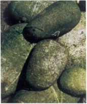 |
 |
 |
| Medium (0.5 to 3 mm thick) | 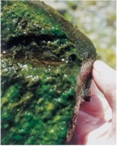 |
 |
 |
| Thick (more than 3 mm thick) | 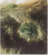 |
 |
 |
| Filament length | Green | Brown/Reddish |
|---|---|---|
| Short (less than 2 cm long) | 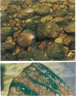 |
 |
| Long (more than 2 cm long) | 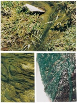 |
 |
Appendix 3 - Cleaning Diatom Samples and Making Slides
Introduction
The identification of diatoms to the species level requires the diatoms to be free of all organic matter, leaving only the silica frustule (shell) behind. Once the diatoms are clean, the sample can be mounted on slides and taxa identified. The method recommended below to clean and mount diatoms has been modified from Lowe and LaLiberte, 2007.
Equipment List
- Diatom samples preserved in Lugol’s
- 1000 mL beaker for each sample
- Tall 200 mL beaker for each sample
- 100 mL graduated cylinder
- Micro-spatula
- Aspirator or large syringe
- Cleaned slides
- Cleaned cover glasses
- Slide labels
- 30% Hydrogen peroxide (H2O2)
- Potassium dichromate (K2Cr2O7)
- Distilled water
- Hotplate
- Small forceps
- Fume hood
- Pipette
- Eye protection
- Gloves
- Lab coat
- High refractive mounting medium (Naphrax or Hyrax)
Slide Preparation Steps
This process must be performed in a fume hood or outdoors with plenty of ventilation
- Transfer 10 mL of the diatom sample into a 1000 mL beaker using a pipette.
- Add 80 mL of 30% H2O2 and allow the sample to stand for at least 24 hours.
- This step should be completed using a fume hood or in a well ventilated outdoor area. Set hotplate temperature to no more than 200°C. Place sample beaker on hotplate, then add a micro-spatula of K2Cr2O7 to the sample.
When the reaction is complete the solution will change from purple to a golden colour. Leave sample beaker on hotplate until this colour change is achieved (this may take from 30 seconds to 5 minutes).
Warning: This will cause a strong exothermic reaction! Be careful that the sample does not bubble out of the beaker!
- Transfer the solution to a tall 200 mL beaker and then add distilled water until the beaker is nearly full.
- Leave the sample to settle for at least 4 hours (settling overnight is preferred). The cleaned diatoms will settle to the bottom.
- After the settling period, carefully remove the liquid at the top of the beaker using an aspirator or syringe. Leave 30 mL of liquid at the bottom of the beaker. do not disturb or remove the sediment/diatom mixture near the bottom!
- Add more distilled water until the sample beaker is again nearly full.
- Repeat steps 5 and 6 until the (remaining) solution is colourless.
- Remove the liquid again, leaving 30 mL at the bottom. Using a pipette, remove some of this concentrate, add a few drops onto 3-6 alcohol cleaned cover glasses and let air dry. (You can place them in a Petri dish and add a label to the dish to keep track of samples).
- Place a drop of mounting medium on a clean slide, then invert the dried cover glass on top. Make sure it is the side with diatoms that goes onto the mounting medium.
- Using the hotplate, heat the slide on the high setting for 30 seconds or until the bubbling slows. This step must be done in the fume hood or outdoors.
- Remove slide from hotplate using forceps. Set down and very gently apply pressure with the forceps to the cover glass to force out the air bubbles.
- Allow the slide to cool, then add a label with site code, date and slide number.
Appendix 4 - Counting and Identifying Diatoms
Introduction
Diatom identification is based on the shape and unique features of the diatom frustule. Distinguishing the different species requires the use of a light microscope (with either brightfield or phase contrast settings) and a 100× oil immersion objective lens to achieve 1000× magnification.
You will identify the first 400 diatom valves you see on your slide, identifying every diatom in your field of view before moving the slide and starting a new field of view. Once you have identified the 400th valve, continue to identify and record the remainder of valves in the current field of view.
Figure 1: Field of View: the area on your slide that is visible when you look through the eyepieces. Before moving the slide you must identify all the diatoms you see within the circle.
Equipment List
- Diatom slides made following the methods in Appendix 3
- Compound microscope with at least 1000× magnification (including 100× oil immersion objective, bright field or phase contrast setting, and a grid for measuring frustules)
- Immersion oil
- Diatom species list and bench sheet
- Diatom identification keys
- Microscope camera (or small digital camera)
- Pencil
Sample Identification Steps
- Place slide on microscope stage and starting near top left corner, locate diatom frustules on slide.
- Focus your samples in the lower magnification range (2×, 4× or 10×) then increase magnification, but not up to the 100× objective.
- Before increasing magnification using your 100× objective, place drop of oil on slide where light shines up through slide. Move 100× objective lens into oil without letting other objectives touch the oil (if they do, clean them off immediately)
- Using diatom identification keys, identify all of the frustules in the first field of view. Remember to count each frustule (diatom half) as one individual. A girdle view, which would show both frustules, would count as two individuals!
hint: certain genera often show up in girdle view: Gomphonema, Pinnularia, sometimes Nitzschia, Navicula and Fragilaria as well.
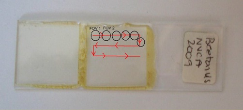
- Move the stage horizontally until you get a new field of view. It helps to start your identifications at one end of the slide and continue to move in one direction only (i.e. left to right), so that you don’t double count any valves. When you get to the opposite end of the slide move up/down and continue.
Figure 2: Moving your slide from one field of view to the next (FOV1 to FOV2)
- Take photos of each new species you identify, or when you find a valve or girdle view that you cannot identify. If you don’t have a microscope camera you can carefully take a photo through the eyepiece using a handheld digital camera. Record the photo number and species name so you can confirm your identifications later.
- Continue identifying all the valves in each field of view until you reach 400 valves. Finish identifying all the valves in that field of view as well.
Recommended Diatom Keys for Southern Ontario include:
- K. Krammer and H. Lange-Bertalot. 2000-2008. Süßwasserflora von Mitteleuropa series (volumes 1 to 5). Spektrum Akademischer Verlag, Berlin
- I. Lavoie et al. 2008. Guide d’identification des diatomées des rivières de l’Est du Canada. Presses de l’Université du Québec, Québec.
Appendix 5 – Data Analysis
After identification of the diatoms to species level, you are now able to use a set of biological indices to evaluate biological conditions. Several different indices for evaluating community composition are listed below (Stevenson and Bahls 1999).
| Taxonomic Composition | Ecological Condition | Sensitivity and Tolerance |
|---|---|---|
| Number of algal species (Species Richness) | % acidophilic diatoms | Pollution tolerance index for diatoms (PTI) |
| Number of genera | % alkaliphilic diatoms | % sensitive diatoms |
| % dominance (for diatoms and for all taxa) | % halophilic diatoms | % motile diatoms |
| Diversity e.g. Shannon Index | % eutraphentic diatoms | % Achnanthes minutissima |
| Eastern Canadian Diatom Index (IDEC) | % oligotraphentic diatoms | % live diatoms |
Given that each monitoring program may have different goals or questions to answer, it is recommended that you use several of the above metrics. At a minimum, species richness, diversity and the Eastern Canadian Diatom Index (IDEC) should be calculated. Using a larger set of metrics will allow for a more complete analysis of the community and will provide a better indication of water quality.
Canonical Correspondence Analysis
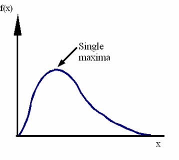
Canonical Correspondence Analysis (CCA) is a common analysis method used to illustrate the relationship between biological communities and environmental variables. This method assumes that species respond in a unimodal fashion along environmental gradients (Figure 1). CCA uses ordinations, a method which arranges site and/or species data along environmental gradients.
Figure 1: Unimodal species response
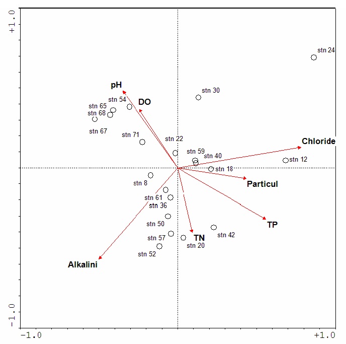
Ordinations created by CCA plot the sites and/or species as points on a graph. Environmental variables are represented by ordination vectors where the length of the arrow indicates the importance or influence of that variable on the biological community. The ordination in Figure 2 plots the diatom communities from monitoring sites across southern Ontario. At these sites the most influential water quality variables are chloride and alkalinity, followed by total phosphorus and pH.
From the ordination diagram, one can infer which environmental variables are strongly differentiating among the sites and species. Sites closest to an ordination vector are most influenced by that environmental variable. In the example illustrated in Figure 2, station 12 is a site located downstream of the QEW highway on Etobicoke Creek. The diatom community there is influenced by high chloride and particulate concentrations. Station 42 is downstream of a wastewater treatment facility; this site has a diatom community that is adapted to waters with higher nitrogen and phosphorus concentrations and may be impacted by organic pollution.
Figure 2: Example of relationships between diatom communities and environmental gradients
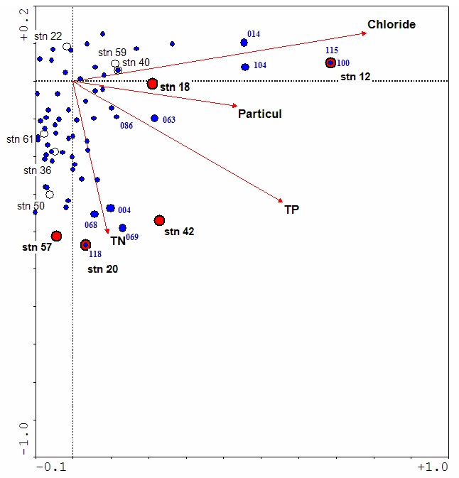
The maximum of each species’ unimodal response is plotted in Figure 3. The distance from each species maximum to each ordination vector indicates how closely the species is associated with that environmental variable. For example, the species numbered 004, 068, 069 and 118 (Achnanthes conspicua, Melosira varians, Meridion circulare and Nitzschia sigmoidea, respectively) are all closely associated with higher total nitrogen concentration. Some of these species are found in eutrophic streams and are also considered indicators of organic pollution (Wehr and Sheath 2003). Species 063 (Gomphonema parvulum) is strongly correlated with total phosphorus, and is an indicator of eutrophic streams.
Figure 3: Relationship between environmental gradients and species optima
Eastern Canadian Diatom Index
The Eastern Canadian Diatom Index (IDEC) was developed using a correspondence analysis (CA) which plotted species optima along a gradient. It is “chemistry-free” in that it does not require any knowledge of the water quality or other environmental variables. IDEC Scores are determined for test sites by the position of each site along the first axis and then adjusted to a scale between 0 and 100. This scale represents how different each diatom community is from its expected reference community, with impacted sites being scored lower. It is assumed that the diatom community at each site is largely influenced by the integration of water quality changes and pollution, and therefore the gradient in the first axis of the CA represents the overall pollution gradient in eastern Canadian streams.
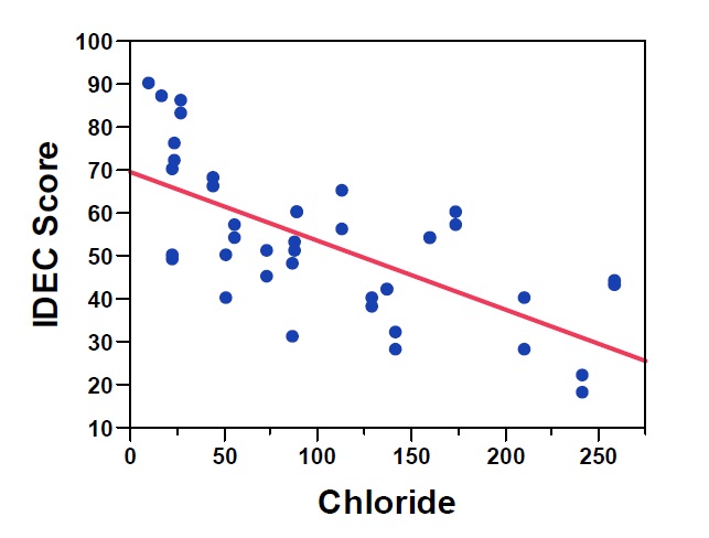
Initial studies in Quebec found that IDEC scores were best correlated with the average water quality calculated over one to five weeks (Lavoie et al. 2008). Application of the IDEC in eastern Ontario streams has revealed strong correlations with nutrients, especially phosphorus (Figure 4), and other water quality variables such as chloride (Figure 5). However, the index not only provides information related to nutrient concentrations, but rather integrates the full suite of variables affecting water quality including nutrients, conductivity, dissolved organic matter, pesticides and other contaminants. Previous studies of diatom communities in Ontario have also been strongly correlated with these types of environmental variables (total nitrogen, total phosphorus, conductivity and metals), supporting the use of an index like the IDEC which evaluates the integrated response of the diatom community to the complete water quality gradient.
Figure 4: Two month average TP (µg/L) vs. IDEC score; R2 = 0.230, p < 0.01
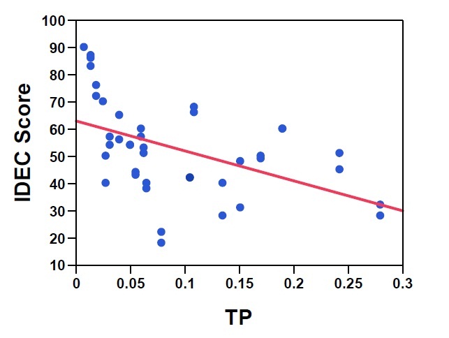
Figure 5: Three month average chloride vs. IDEC score; R2 = 0.455, p < 0.0001
The utility and merit of the IDEC has been recognized by the Quebec Ministry of the Environment, which uses diatom assessments as part of its watershed assessments. The IDEC is used alongside other monitoring programs that evaluate watershed health based on water chemistry and benthic invertebrates. Both water chemistry and benthic invertebrates have been well correlated with the IDEC scores in these programs. In 2009, 50 watershed assessments were conducted on agricultural streams prior to restoration activities (Isabelle Lavoie, personal communication). As a cost savings measure, the sites were screened based on their IDEC scores so that expensive water chemistry analyses were not necessary for all sites. Detailed chemical analysis and subsequent restoration efforts were then focused on those streams that were identified as being impaired during the IDEC analysis. As of 2011, over 100 streams in eastern Canada have been evaluated using the IDEC (Lacoursière et al. 2011) and the index is currently being updated with data collected in southern Ontario streams. The new version will be suitable for widespread application in Ontario.
Examples of watershed assessments using IDEC:
- Pelletier, D., 2008, État de l’écosystème aquatique du bassin versant de la rivière Kamouraska: faits saillants 2004-2006, Québec, ministère du Développement durable, de l’Environnement et des Parcs, Direction du suivi de l’état de l’environnement, ISBN 978-2-550-52168-6, 12 p.
- Beauchamp, M. and Simard, A., 2007, État de l’écosystème aquatique du bassin versant de la rivière du Nord : faits saillants 2004-2006, Québec, ministère du Développement durable, de l’Environnement et des Parcs, Direction du suivi de l’état de l’environnement, ISBN 978-2-550-51585-2, 14 p.
The IDEC is recommended for analysis of the diatom communities collected following the ABP. There are many other metrics available; however, many of them were developed outside of Ontario and North America. While these other indices do provide a valuable assessment of water quality, the reference conditions upon which index criteria were derived may not apply to Canadian conditions. For this reason it is recommended that the IDEC be used when analyzing diatom samples, and that the other diatom indices be used for supplementary analyses.
References for statistical analysis
Jongman, R. H. G., ter Braak, C. J. F., van Tongeren, O. F. R. 1995. Data Analysis in Community and Landscape Ecology. Cambridge University Press.
The Ordination web page. Ecology at Oklahoma State University.
ter Braak, C. J. F. 1987. Ordination. In: Jongman, R.H., C.J.F. ter Braak and O.F.R. van Tongeren, editors. Data Analysis in Community and Landscape Ecology. Wageningen, The Netherlands: Pudoc. pp. 91-173
ter Braak, C. J. F., and I. C. Prentice. 1988. A theory of gradient analysis. Adv. Ecol. Res. 18:271-313.