Lakeshore Capacity Assessment Handbook: Protecting Water Quality in Inland Lakes on Ontario’s Precambrian Shield Appendix C : Dorset Environmental Science Centre Technical Bulletins
This document provides Dorset Environmental Science Centre Technical Bulletins.
May 2010
Ministry of the Environment
Environmental Sciences & Standards Division
Standards Development Branch
40 St. Clair Avenue West
Toronto, Ontario M4V 1M2
Strategies and Parameters for Trophic Status and Water Quality Assessment
Trophic Status
The concentration of nutrients (phosphorus and nitrogen) in a lake directly influences algal growth, water clarity, and other in-lake processes such as hypolimnetic oxygen depletion and growth of near-shore periphyton and rooted aquatic plants. The evaluation of trophic status is, therefore, often a prerequisite to the management of a water body. Evaluation of trophic status is especially important if nutrient loading to the water body is expected to change or if there are recent signs of increased eutrophication.
Trophic status is commonly measured (or monitored) using at least one of three parameters. These are transparency (Secchi depth), chlorophyll a, and total phosphorous (TP) concentration. Dissolved oxygen which is also considered an indicator of trophic status is addressed in another report.
Transparency is a sensitive indicator of long-term changes in trophic status. It has been shown that Secchi disc measurements are less subject to withinyear variability than either chlorophyll a or phosphorous measurements and as such can provide a better monitoring tool for early detection of eutrophication. Transparency observations, however, may be influenced by factors other than those related to trophic status (e.g., dissolved organic carbon (DOC)) and should, therefore, be interpreted together with TP and/or chlorophyll a data, especially for between-lake comparisons.
Chlorophyll a often is collected as an indicator of trophic status primarily because a change in algal biomass is the most evident result of a change in the trophic status of the lake. Chlorophyll a, however tends to show a great deal of seasonal and inter-annual variation, especially in more eutrophic systems. As these seasonal patterns cannot be represented by a single or even several observations, it is often necessary to collect numerous samples throughout the year to determine meaningful 'ice free average' concentrations. It is, on average, necessary to collect more than 10 samples per season to derive averages which are within 20% of the seasonal mean (95% confidence) and 30 to 50 samples to be within 10% of the seasonal mean. Based on data from Dorset lakes, establishing a longterm mean will require one to four years of data collection to be within 20% of the long-term mean and three to 16 years to be within 10%. Generally, the more eutrophic the system the more years of data that will be required. In addition, chlorophyll a samples tend to be perishable and very susceptible to a number of 'handling' problems between the time of sampling and analysis of the sample. While there may be merit in quoting individual chlorophyll a concentrations to quantify the extent of an algal bloom or to indicate how high or low concentrations are in general, it is both costly and labour-intensive to use chlorophyll as a tool to reflect trophic status.
Total phosphorus, the basis for most trophic status models, including the MOEE Lakeshore Capacity Model, is the most reliable indicator of trophic status. Average TP concentrations in a lake can be estimated by measuring a single spring turnover concentration and long-term average numbers can be determined with the collection of only several years of turnover data. Two years of data records will provide results within 20% of the long-term mean (95% confidence), but approximately seven years are required to be within 10% of the long-term mean (provided the lake is not undergoing significant changes in nutrient level). Some researchers report' ice free average TP concentrations' which require the collection of up to ten samples each year and the use of volume-weighted distinct 'layer' samples while the lake is stratified. These observations will yield reliable long-term averages in fewer years than spring turnover samples, but this advantage generally does not justify the extra effort required to collect the data. The recommended method for determining the trophic status of a lake is therefore based on the collection of spring overturn TP data over several years. These are usually collected as composites of the top 5 m of water at the deepest location in the lake. Samples are best collected after the lake has had an opportunity to mix for several days (temp > 4°). Thermal stratification may occur rapidly after turnover, but chemical stratification does not occur as quickly so that surface TP concentrations are usually similar to spring overturn concentrations for several weeks after thermal stratification occurs. Generally, spring TP concentrations can be collected any time when surface water temperatures are between 5 and 10°. Caution is required with respect to the type of sample containers used. Details of this concern and outlines of other sampling protocols can be obtained by contacting the Dorset Research Centre.
Field programs that require staff to visit a lake several times each year (at least monthly) would also benefit by collecting Secchi disc observations at each visit. This would allow the addition of 'ice free average' transparency data to the database which would allow the observation of long-term trends in trophic status.
Water Quality Assessment
It is desirable to collect water quality data to describe chemical or physical characteristics of a lake for reasons other than trophic status. Concerns over acidification, for example, require the collection of pH, alkalinity, sulphate, and other related parameters. When comparative studies are undertaken, it is useful to group lakes on the basis of concentrations of major ions or to distinguish the dystrophic (brown water) lakes in the data set by observing DOC or colour. Each research related use for the database may require the collection of additional parameters and it may become difficult to choose tests that both fulfil the current project needs and provide background information for future research.
Parameters collected by the Ministry of the Environment and Energy (MOEE) which can be used as a guideline for describing the general water quality of a water body include: pH, alkalinity, total Kjeldahl nitrogen, nitrate, ammonia, iron, conductivity, colour, dissolved inorganic and organic carbon, calcium, sulphate, and total phosphorus. Secondary parameters collected less often include: aluminum, fluoride, manganese, chloride, potassium, magnesium, silica, and sodium.
Similar to the sampling strategies outlined for the determination of trophic status, these parameters can be measured with minimal effort at spring turnover with 5 m composite samples. The data obtained from a single visit when the lake is 'mixed' will be more valuable than several years of data that may include several visits per season if those sample dates are at times when distinct samples do not represent the whole lake. Small lakes will require measurements at only one mid-lake station while large lakes or lakes with localized influences may require the establishment of several sampling locations More extensive collections of information from distinct layers during stratification or at other times of the year will only be necessary if specific, complex interpretations are required.
The number of years of water quality data that are required is parameter specific. The use of a single number for complex analysis or for input to models should consider between year or seasonal variability on a parameter by parameter basis. It is, however, common to accept the water quality description of a water body based on the results of the most recent visit without concern for the year to year variance associated with the individual parameters.
Sample container and submission protocols vary with each parameter and should be verified through contact with MOEE labs or by contacting MOEE field staff at the Dorset Research Centre.
For further information, contact:
B. Clark
Email: clarkbe@ene.gov.on.ca
Hypolimnetic Oxygen: Data Collection Strategies For Use In Predictive Models
Data Collection Strategies For Predictive Models
Hypolimnetic oxygen concentrations are a key element of habitat quality for many cold-water species. These include fish such as lake trout and whitefish as well as many invertebrates including Copepods and Mysis that are important food for fish. Oxygen concentration profiles are typically measured at the deepest location in the lake, usually on a monthly basis throughout the open water season. These types of data are difficult to interpret because concentrations change both spatially and temporally in a specific year and also tend to show considerable inter-annual variation.
One method of addressing a great deal of this variation is to examine only end-of-summer or end-of-stratification oxygen profiles. This eliminates the need to evaluate seasonal changes in the profile and concentrates on the “worst case” profiles at the time of year when oxygen concentrations in the hypolimnion are at the open- water minimum. When attempting to characterize lakes in this manner, it is preferable to use average profiles which are derived from several years of data to offset the effects of inter-annual variation. This approach will allow the description of average conditions in a lake’s hypolimnion at the end of summer (early in September) and compare between-lake differences under similar conditions.
In 1992, a model* which predicts steady state, end-of-summer oxygen profiles for small oligotrophic lakes was developed as an additional component of the ministry’s Lakeshore Capacity Model (LCM). The oxygen model uses lake morphometry and epilimnetic phosphorus concentration to predict end-of-summer oxygen concentrations of each stratum in the hypolimnion. An example is shown in Fig. 1. The model requires total phosphorus (TP) as one of its parameters, and can therefore be used to predict the effects of shoreline development on hypolimnetic oxygen.
Recent efforts to validate the model indicate that it will predict end-of-summer profiles for lakes with a broader range of size and trophic status than those that were used to formulate the model.
Morphometry plays a major role in determining hypolimnetic oxygen concentrations. With the model, oxygen profiles can be predicted using as a minimal, a lake morphometric map and a modelled TP value (if no measured TP data exist). It is preferable to use long-term mean spring overturn TP.
To use the model for predicting the effects of changes in trophic status, it is preferable to average several years of oxygen profiles from the time period spanning two weeks either side of the first week in September. The model is then used to predict how changes in TP concentrations would effect the measured (not modelled) long- term average profile. This approach maintains the unique shape and magnitude of the lake’s end-of-summer oxygen profile. Operation of the model is straightforward and it can be obtained as a spread sheet from the Dorset Research Centre.
From a data collection standpoint, this approach to oxygen monitoring suggests that field crews concentrate on the collection of end-of-summer profiles specifically between August 15 and September 15. Temperature profiles should also be collected to determine hypolimnetic boundaries. Data bases, for example, could benefit more from the collection of oxygen profiles from several different lakes circa early September than from a series of monthly observations from the same lake over the course of a summer. In other words, in this case, a survey approach would be more useful than a monitoring program.
Determining Hypolimnetic Volume-Weighted Oxygen Concentration
There are several methods used to quantify cold-water fish species habitat based on oxygen concentrations. For lake trout, optimal habitat has been described as having greater than 6 mg·L-1 oxygen at less than 10°C. Usable habitat has expanded boundaries at greater than 4 mg·L-1 oxygen and less than 15°C. These guidelines can be used to generate habitat guidelines can be used to generate habitat interpret since similar “volumes” between lakes may represent different proportions of total lake volumes.
The proposed use of end-of-summer, volume-weighted hypolimnetic oxygen concentrations to define lake trout habitat would eliminate many of these problems. Lakes with large volumes of oxygenated water would not have their average greatly affected by small volumes of depleted water near the bottom. Lakes with small and enriched hypolimnia would be affected to a greater degree by increased depletion in bottom waters. It is suggested for lake trout that these values remain above 7 mg·L-1 oxygen.
Calculating volume-weighted hypolimnetic oxygen requires morphometric data and at least one end-of-summer oxygen profile (Aug 15 - Sept 15 ). Ideally, oxygen profiles from several years would be used to reflect long-term average conditions. Area and depth information from morphometric maps should first be converted to ha and m if originally in acres and feet. This will yield contour areas in ha for uneven numbers of m but these can be converted to 1 or 2 m contour areas by one of two methods:
- Metres and ha are plotted and the individual areas for each stratum are simply read from the axis of the graph.
- Individual pairs of adjacent points in ha and m are used to interpolate areas for the intervals that fall within the depth range spanned by the pair of points. This can be done through simple linear interpolation or by doing a linear regression on two pairs of points. However, it is important to note that entire sets of hypolimnetic depth/area data cannot be regressed as a single group of numbers because the relationship is almost always curvilinear. Individual contour areas are then converted to volumes by the formula:
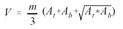
Where:
- V
- is volume in m3 × 104
- At
- is the area in ha of the top of the stratum
- Ab
- is the area in ha of the bottom of the stratum
- m
- is the depth of the stratum in m
The volume of each stratum of the hypolimnion is then expressed as a fraction of the total hypolimnetic volume and multiplied by the oxygen concentration observed for that stratum. These individual concentrations are summed to yield volume-weighted average oxygen as shown in the example below.
| Stratum | Volume (103m3) | A-Volume as fraction of total Volume | B-Dissolved oxygen (mg·L-1) | A * B |
|---|---|---|---|---|
| 14-16m | 1500 | 0.49 | 10.0 | 4.9 |
| 16-18m | 1000 | 0.33 | 8.0 | 2.6 |
| 18-20m | 400 | 0.13 | 6.0 | 0.78 |
| 20-22m | 150 | 0.05 | 1.0 | 0.05 |
Total of A * B is volume weighted oxygen concentration 8.33
It should be noted that volume-weighted oxygen concen-tration calculations yield a single number which may respond differently from lake to lake to changes in trophic status. The number should be interpreted together with other physical and chemical information relating to the lake in question. However, it is a simple and useful measure related directly to lake trout habitat.
* Details of the oxygen model have been published in: Molot, L.A., P.J. Dillon, B.J. Clark, and B.P. Neary. 1992. Predicting end-of-summer oxygen profiles in stratified lakes. Can. J. Fish. Aquat. Sci. 49:2363-2372.
For further information, contact:
B. Clark
Email: clarkbe@ene.gov.on.ca
The Trouble With Chlorophyll: Cautions Regarding The Collection And Use Of Chlorophyll Data
Resource managers and researchers from many agencies commonly use chlorophyll as a trophic status indicator. Although variation in chlorophyll concentration tends to be the most evident consequence of changes in trophic status, there are problems involved with using this test as a basis for either setting trophic status objectives or detecting long-term change. These problems can be summarized as follows:
- the collection and submission of chlorophyll samples require precautions that are complex compared to other trophic status parameters
- changes in analytical methods may disrupt long-term chlorophyll data sets.
- significant seasonal and inter-annual variation in chlorophyll requires the collection of large numbers of samples over many years.
- many different chlorophyll pigments are commonly measured, i.e.: Chl a, b, c, chl a corrected etc., concentrations of these pigments may not correspond to actual phytoplankton cell densities.
Data Collection
Chlorophyll samples must be collected into opaque bottles and immediately fixed with magnesium carbonate (MgCO3 ensures that the sample remains ‘basic’ to avoid conversion of primary pigments to phaeopigments under acidic conditions). They must then be kept cool and filtered as soon as possible. The filtrate must be frozen and transported to the lab without being allowed to thaw. This makes the remote collection of samples difficult or impossible such that, from the onset, chlorophyll data can present uncertainties if the samples have not been collected under strictly controlled conditions.
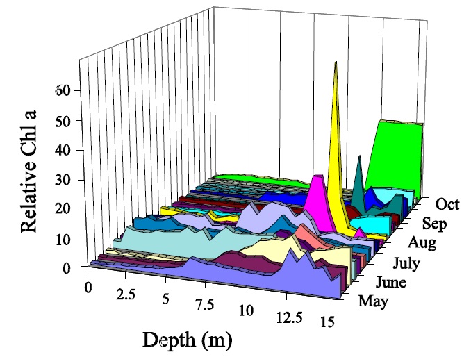
Chlorophyll samples are often collected as euphotic zone composites and reported as ice-free means. The euphotic zone, usually approximated as twice the Secchi disc visibility, is sometimes well mixed since much of this layer is composed of epilimnion. However algal cells will often stratify dramatically below the epilimnion and this can occur even in mixed layers (Fig.1). This means that chlorophyll concentrations based on euphotic zone composite samples may vary based simply on the physical collection methods i.e.: how the water is combined in proportion from given depths. This is very relevant in situations where the depth of the euphotic zone relative to the thermocline changes over time.
Figure 1: Vertical distribution of Chl a in Plastic Lake.
Changes in Analytical Methods
The reported concentrations of chl a have been subject to methods changes at the MOEE laboratories. The long-term data base has been most notably broken due to changes in the methods that occurred in 1985. At that time, a switch to nylon filters increased extraction efficiencies of the acetone. This resulted in an increase in post ‘85 values. Although it may be possible to ‘align’ the data before 1985 to match current values, there is no single correction factor that can be applied to these data. Data base managers who have chlorophyll values spanning 1985 should refer to the documentation referring to the methods changes which was published by the Lab Services Branch in 1985.
Seasonal and Inter-Annual Variation
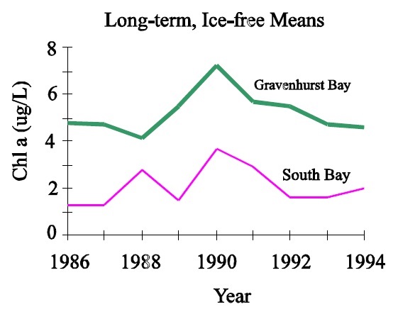
The largest problem with the interpretation of chlorophyll data is associated with seasonal and inter-annual variation. Chlorophyll concentrations vary significantly on a seasonal basis within lakes and often show different seasonal patterns between lakes (Fig.2). In addition there is a great amount of long-term, or between-year variation in the ice-free means for individual lakes. (Fig.3) This makes it necessary to collect numerous samples each year to derive ice-free means that are close to the actual value, and many years of this type of data are required to estimate the long-term mean (Table 1). Thus it is difficult to assess whether observed changes in chlorophyll are actually reflecting long-term change or whether they are simply noise based on the collection of too few samples each year or too few years of data being used to detect the change. Development objectives for individual lakes that are based on chlorophyll will therefore be difficult to assess since it will be imposible to tell the difference between the actual surpassing of objectives and simple variation based on the collection of too few samples. These problems tend to increase in severity with increasing trophic status such that the situations that require the most attention, i.e.: more enriched systems, also tend to require the most samples to describe accurately.
Figure 2: Seasonal changes in chl a for Gravenhurst Bay, Chub, Dickie and Red Chalk lakes in 1993.
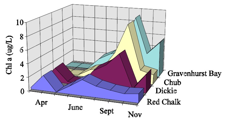
Figure 3: Long-term variation in ice-free Chl a for Gravenhurst Bay and South Bay (Lake Muskoka).
| % of mean | # samples/year 10 | # samples/year 20 | # samples/year 50 | # years 10 | # years 20 | # years 50 |
|---|---|---|---|---|---|---|
| Blue chalk | 55 | 14 | 2 | 3 | 1 | 1 |
| Harp | 59 | 15 | 2 | 7 | 2 | 1 |
| Dickie | 126 | 32 | 5 | 16 | 4 | 1 |
Cell Density VS Pigment Concentration
Finally, the whole picture is further complicated by the fact that chlorophyll concentrations are not always tied to phytoplankton cell densities. The actual concentration of chlorophyll in algal cells is determined by incident radiation, species composition, nutrient supply and certain aspects of algal physiology. These determinants have a seasonal component such that the correspondence between chlorophyll a and algal cell densities is not constant. These relationships can further be specific to different chlorophyll pigments. In most cases chlorophyll a or a version of chlorophyll a corrected for phaeopigments is used to represent the phytoplankton community. Sometimes chl b or chl c are quoted but often the relationship between the concentrations of specific pigments and the concentrations of algal cell in the lake do not correspond because the cells in greatest abundance do not contain pigments that are being measured. Also, algal communities are changing seasonally back and forth between those that contain the investigator’s pigment of choice and those that do not.
Conclusions and Recommendations
When all of these problems are considered it makes it difficult to recommend chlorophyll as a trophic status indicator in situations where small amounts of data are collected. Most of the problems outlined above are amplified by the collection of too little data. This is not to say that chlorophyll data should not be collected. A great deal of usefull data exists that show the effects of phosphorus load reductions, zebra mussels, etc. on chlorophyll concentrations. These are generally based on large data sets that are not plagued by seasonal or inter-annual variation.
Since virtually none of the same problems outlined for the collection of chlorophyll data apply to the collection of total phosphorus data it is probably better to use total phosphorus as an indicator of trophic potential in situations where minimal data sets are being collected.
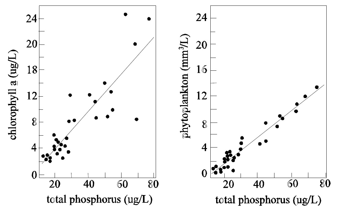
Lastly, the cost of monitoring the trophic status of a lake based on spring turnover TP would be a fraction of that involved with using chlorophyll. Spring turnover total phosphorus based trophic status estimates would require only one visit to each lake per year. Since ice-free mean chlorophyll estimates require at least 6 or 7 visits per year and considering that the chlorophyll test is approx 4 times as expensive as a TP test, the relative difference in test costs alone would be in the neighbourhood of 25 times. When staff and transportation costs are considered the numbers become significantly different. Cost aside, the results would be much more reliable when based on total phosphorus such that it would be recommended in almost every case to base trophic status estimates on total phosphorus. If information about the phytoplankton community must be collected, managers should consider collecting seasonal composite phytoplankton enumeration samples. Generally, weekly, bi-weekly or monthly phytoplankton samples are collected and fixed with Lugols fixative. These may be combined at the ennumeration Lab in Rexdale and counted to provide seasonal, mean, phytoplankton cell densities. These numbers will relate better to trophic status than will chlorophyll estimates (Fig.4) and the costs will still be approximately half.
Figure 4: Relationship between total phosphorus and chlorophyll a (left) and phytoplankton cell volume (right).
Details about estimating the trophic status of a lake based on total phosphorus are available in STB Tech. Bull. DESC-4.
For further information, contact:
B. Clark
Email: clarkbe@ene.gov.on.ca
Long-Term Monitoring Of Trophic Status: The Value Of Total Phosphorus Concentration At Spring Overturn
There are many reasons to measure the nutrient status of a water body. It may be done as part of an initiative to control nutrient inputs in an effort to reduce nuisance levels of aquatic plants or algae. In some cases, measurements are taken as part of a self-regulation program designed to monitor inputs to surface waters. In most cases, however, the nutrient status of a water body is measured to detect long-term changes in water quality (the nutrient status) of the water body.
The three most common measures of the nutrient status of a water body are TP (total phosphorus), chlorophyll a and Secchi depth. In Ontario, Secchi depth is often controlled by DOC rather than by chlorophyll and the chlorophyll measurements themselves are costly and must be pooled in large numbers to yield meaningful icefree means (see Techbull DESC_ 10 ). For these reasons, TP is the recommended parameter to monitor long-term changes in trophic status. This is supported by the fact that TP is almost always the limiting nutrient for algal growth in Ontario lakes. In addition, TP surveys are easy and comparatively inexpensive to conduct.
Once the decision has been made to monitor long-term changes in TP, decisions must be made with respect to the type of sampling regime that will be followed. Since seasonal variation in TP would rarely be of interest, it is, in most cases, desirable to obtain some number that describes an annual average condition such that the individual annual means can be monitored through time.
There are many different ways to combine TP samples to derive some measure of an annual mean. Monthly samples can be pooled to derive an "ice-free mean" but care must be taken when combining these numbers to produce "means" that can be validly compared to the numbers derived by similar studies elsewhere. For example, individual surface water samples when taken as 5 metre composites or euphotic zone composites when pooled will give an ice free epilimnetic or euphotic zone (annual) mean. This number will be different from numbers generated by other programs that volume weight the stratified season samples taken from all layers of the lake to accurately produce a "whole-lake" ice free annual mean. For these reasons it is often safer to collect TP samples at spring overturn to detect long-term trends. Certainly, it is better to have a single, reliable spring-overturn number than it is to average several samples that have been collected in a helter skelter fashion at other times of the year. The DESC database clearly shows that long-term average TP concentrations derived for a given lake using spring turnover samples are very closely corelated to those derived using icefree means by volume weighting. (Fig 1).
TPif = 0.96TPso + 0.31
r2 = 0.93
Fig. 1. The relationship between long term mean TP derived using spring turnover and ice-free mean data for the lakes in the Dorset database.
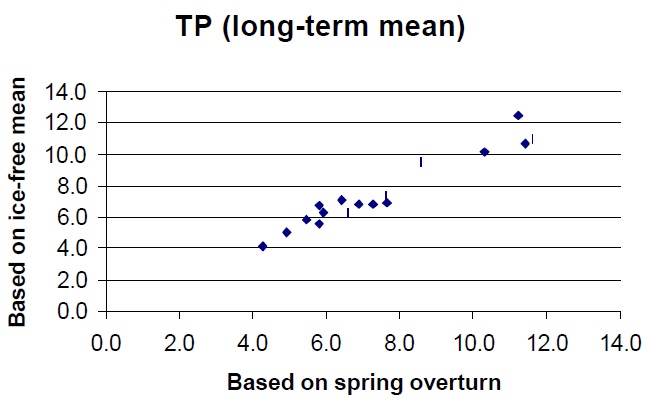
Note: Volume weighting is used to collect data for all parameters for use in mass balance calculations at the DESC and probably would not be conducted if the only goal was to monitor changes through time in whole lake TP concentrations.
Previous calculations based on DESC data have shown that a reliable long-term mean can be derived with 2-4 years of spring turnover data. The ice-free, volume-weighted means will provide a reliable long-term mean sooner i.e., within 1-3 years but the extra effort and cost is usually not justified. In fact, for many lakes, the long-term trend is described as well or better by spring turnover TP than by ice-free volume weighted means (Fig 2).
Fig.2. Annual TP expressed as spring overturn concentrations and as ice free means ( mean of monthly volume weighted concentrations) for Blue Chalk Lake.
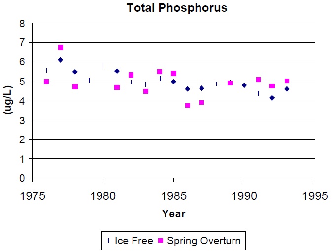
Fig.3. The 5m composite sampling method.
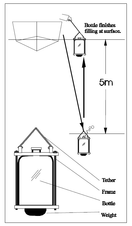
Spring turnover TP concentrations should be taken as some form of surface water composite (i.e., 5m composite bottle sample) from the deepest location in the lake (Fig.3.). Ideally the sample should be taken a week or so after ice out to allow the lake to completely mix. Samples should be taken, however, before water temperatures reach ~10°C. It is not acceptable, to include values in the database that are collected outside this window. It should also be noted that a single spring TP sample will not be adequate to describe the conditions that occur in complex systems such as;
- in very large lakes
- where large inflows dominate the nutrient concentrations in the lake
- in eutrophic lakes where there are large nutrient fluxes or a high degree of spacial variation
- in lakes where anthropogenic loads are high such as in lakes that adjoin urban centres.
For more information, contact
Bev Clark, DESC, 705-766-2150
Email: clarkbe@ene.gov.on.ca