Ontario specification for Global Navigation Satellite Systems (GNSS) geodetic control surveys
Learn how to establish GNSS networks for inclusion in the provincial geodetic reference framework in COSINE.
Introduction
This document provides the minimum requirements when undertaking a Global Navigation Satellite Systems (GNSS) Geodetic Control Surveys in Ontario. This specification is intended for use in medium-scale GNSS control surveys (for example, municipalities, highways, pipelines) where typical station spacing is 1 km or greater. This specification provides the requirements for establishing two and three dimensional GNSS networks for integration into the provincial geodetic reference framework held within the provincial geodetic database, the control survey information exchange, more commonly referred to as COSINE. This document is divided into the following sections:
- Section 2 provides the minimum requirements for a horizontal or 2D GNSS network to meet provincial specifications for integration into the official horizontal datum of Ontario.
- Section 3 provides the minimum requirements for a 3D or vertical (1D) GNSS network to meet provincial specifications for integration into the official horizontal and vertical datums of Ontario.
- Section 4 describes the required project deliverables, and the appendices provide information related to monumentation, sample network design, field notes and sample orthometric height accuracy calculations.
Contacts
Ministry of Transportation of Ontario (MTO)
Geomatics Office
301 St. Paul Street, Floor 2
St. Catharines ON L2R 7R4
Tel:
Ministry of Natural Resources (MNR)
Geodetic Services Team
Office of the Surveyor General
300 Water Street, 2nd Floor North
Peterborough, ON K9J 3C7
Tel:
geodesy@ontario.ca
2D/Horizontal GNSS Control Survey
Horizontal accuracy of the network
The local or relative accuracy of the network is determined by averaging the semi-major axes of the horizontal relative confidence ellipses, at the 95% confidence level, from a weighted constraint adjustment, for all connected stations, whose weights are determined from the provincial weighted station adjustment.
The network or absolute accuracy of the network is determined by averaging the semi-major axes of the horizontal station confidence ellipses, at the 95% level, from the weighted constraint adjustment, for all stations.
Both the relative and station confidence ellipses are produced by iteratively rescaling the GNSS baseline covariance information until the final weighted constraint adjustment has an a posteriori variance factor equal to 1.
The classification of local and network accuracy for a survey can fall into groups based on:
- accuracy
- monumentation
- GNSS occupation time
- connection to Primary Interagtion Network (PIN) station
Table 1 specifies the minimum requirements for each class.
Table 1: Station classification – Horizontal
| Class | Horizontal Accuracy upper limit (cm) | Monumentation type and station status | GNSS minimum common session observation time | Connection to PIN or Key station network (KEY) |
|---|---|---|---|---|
| A | 1 | CBN Pillar/CACS/RACS – existing monument | 90 minutes | Mandatory as part of PIN (or KEY) station network |
| B | 2 | Monuments in stable concrete or stable rock structures – existing monument | 90 minutes (if PIN) or 60 minutes (if KEY) | Mandatory as part of PIN or KEY station network |
| C | 3 | Brass cap or rock post in stable concrete or stable rock as per Appendix A – existing or new monument | 45 minutes | Typically, part of KEY station network directly connected to PIN |
| D | 5 | Brass cap or rock post as per Appendix A (preference not to place monuments in sidewalks) - existing or new monument | 30 minutes | Typically, part of project network – stations are not usually directly connected to PIN |
| E | 10 | Brass cap or rock post as per Appendix A - (if there is no alternative, monuments in sidewalks are permissible) - existing or new monument | 30 minutes | Typically, part of project network – stations are not usually directly connected to PIN |
Reconnaissance
Site selection
When selecting suitable locations for new control stations, the following must be considered:
- satellite visibility
- safe access and permanence of monument
- low-multipath environment (there should be no reflective surfaces within 50 m from the station in any direction)
- station locations should be chosen so they are not near microwave transmitting stations, radio repeaters or high voltage power lines
Once the site has been monumented, a monument position sketch and a station obstruction diagram must be made.
Monumentation
Monuments for new control stations shall be one of the following.
- A tapped brass cap affixed to a diecast or machined 1.8 metre or longer, 25 mm diameter round iron bar, driven a minimum of 15 cm below ground level (monument type B and B2). The station must be marked with a 2” x 2” x 4’ wooden stake when possible.
- A brass rock post counter sunk and set flush in stable rock or concrete (monument type C). Stations set in rock must be marked with a steel marker, set in the rock, to aid in locating the cap. A measurement from the marker to the monument must be made and recorded in the monument position sketch.
Monument position sketches
Monument position sketches are required for all new control stations and any existing control stations where reference ties and/or local conditions have changed (for example, road widening, new pavement or new sidewalk). The information needs to be updated when errors and/or omissions are noticed. The reference sketch will indicate the relationship of the monument to the highway or road and show a minimum of 3 other ties to unambiguous references. Ties should be sufficient to locate the object at the decimetre level and include redundant measurements. Poles and trees used as reference ties must be marked with nail and flagging. Also required are:
The reference sketch will indicate the relationship of the monument to the highway or road and show a minimum of 3 other ties to unambiguous references. Ties should be sufficient to locate the object at the decimetre level and include redundant measurements. Poles and trees used as reference ties must be marked with nail and flagging. Also required are:
- a north arrow
- date of ties
- monument type
- stamped number
- condition
- relationship to ground
- intervisibility to other stations
- a written description for rough locating purposes, referencing the monument in both directions to local features such as:
- roads
- rivers
- towns
A sample monument position sketch is given in Appendix B.
Network design
There are 3 main components which together provide for a complete network design:
- The primary integration network (PIN)
- The key station network (KEY)
- The project network
Each component of network design falls under a different control survey hierarchy (figure 1). The primary integration stations are of greater hierarchy than that of the project network. Note that existing key stations can be used for primary integration. The project network falls under the regional control classification.
The network must be designed with inherent quality control checks to ensure the reliability of the survey and the methodology used. The checks will include repeat baseline observations, repeat occupations on both existing and new control stations, and other quality control measures.
Sufficient existing control must be used to allow proper orientation and scale of the project network. The final configuration must be geometrically strong and result in a fully integrated, homogeneous network. Samples of suitable network designs are given in Appendix C.
Figure 1 shows the control survey hierarchy as a pyramid. The gray areas indicate the stations to be produced in the survey. The arrow shows which stations can be used for primary integration.
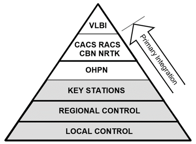
A triangle diagram representing the control survey hierarchy with the lowest level which reads, local control, followed by regional control, key stations, OHPN, CACS, RACS, CBN, NRTK and VLBI at the highest level at the peak.
A network design proposal must be submitted and approved by the issuing agency (see contacts in section 1 of this document) before field observations commence. The network design proposal must include:
- a proposed network diagram showing all new and existing stations
- the baselines to be observed, with session identification
- the baselines which will be repeated
- the number and type of GNSS receivers and antennae
- comments on any element of the proposal that may concern the issuing agency
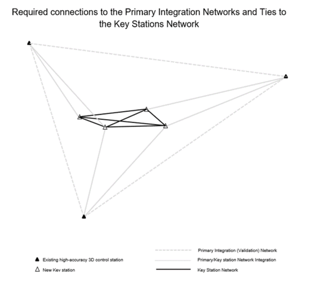
Primary Integration Network (PIN)
The primary integration network provides both the integration to higher order control as well as the overall network structure. Three or more existing control stations distributed regularly on the periphery of, and fully encompassing the project network, must be used. They are to be directly connected to each other, forming a validation network, to provide both quality control and integration for the key station network and project stations.
These stations should be of greater hierarchy than that of the project network. For example, primary integration stations can be previously established key stations, Ontario High Precision Network (OHPN) stations, Canadian Base Network (CBN) stations, Canadian Active Control System (CACS) stations or Regional Active Control Stations (RACS) and private sector Network Real Time Kinematic (NRTK) base stations that are deemed compliant by Canadian Geodetic Survey (CGS) at the time of the survey. No more than 50% of the PIN stations can be private sector Network RTK base stations.
Key Station Network (KEY)
Key stations, when connected to each other and to the primary integration network, provide for a homogeneous network with minimal error propagation. They will form part of the OHPN – the provincial densification of the CBN once a survey is completed and approved for acceptance.
The key station network must form an independent network when combined with the primary integration network.
Key stations are to be set at the periphery and should encompass the project area. They will form part of the project network. For a linear network a minimum of 2 key stations are required. For a block network (a network of square, rectangular or similar shape) a minimum of four key stations are required. Additional key stations are required so that the maximum spacing between key stations is 15 km. They are to be high quality stations, preferably set in stable rock or concrete, and with minimal satellite obstructions.
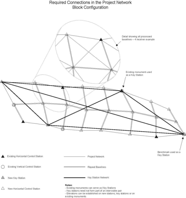
Project network
The project network is the local densification of control stations. Connections to the key station network provide for primary integration and quality control. The configuration of the project network will be dependent on the survey requirements specified by the issuing agency.
Existing horizontal control
In addition to the primary integration stations, other existing horizontal control must be occupied and properly integrated into the network (if they are suitable for GNSS) to ensure a fully integrated, homogeneous project network.
For linear projects, at least 1 existing horizontal control point every 5 km within the project network must be occupied and integrated in a homogeneous manner.
For block projects, at least 25% of the existing horizontal control within the project network must be occupied and integrated in a homogeneous manner.
Existing horizontal control points should form part of the project network where possible.
Station interconnections
The final network must include direct connections between the primary integration network (PIN) stations.
A direct connection is required from each existing control station in the primary integration network, to the 2 closest key stations. These connections must be observed in separate sessions and under a different satellite constellation.
Key stations are to be tied directly together in addition to ties to the Primary Intergration Network and project network.
Each station in the project network (including key stations) must be directly connected to at least 2 other stations in the project network and must have direct connections to all adjacent stations. All intervisible station pairs must be directly connected
Repeated baselines
There must be at least 1 common baselines betweekn sessions so that in the final netowrk, all sessions are tired together.
For linear project networks, all baselines between intervisible station pairs must be repeated.
Repeated occupations
Each station in the GNSS survey, including existing control, must have 2 independent occupations.
Equipment selection
Receiver
A minimum of 4 geodetic quality, dual frequency GNSS receivers must be used. Regardless of the number of receivers being used, all elements of design must be achieved (for example, repeat baselines, common baselines between sessions, ties to adjacent stations).
The use of 1 make and model of receiver is highly recommended.
If receivers from different manufacturers are mixed, their compatibility must first be verified and documented by carrying out a GNSS validation survey on a provincial GNSS basenet.
Antenna
At minimum, dual frequency (L1 and L2) geodetic antennae must be used. The use of 1 make and model of antenna is highly recommended.
If antennae from different manufacturers are mixed, their compatibility must first be verified and documented by carrying out a GNSS validation survey on a provincial GNSS validation network or basenet. The proper application of antenna heights and phase center offsets must be verified in both the baseline processing software and in the header of the Receiver Independent Exchange (RINEX) file.
Field observations
Monument identification
For each occupation, it must be verified that the correct station has been occupied.
The receiver operator must record on the field log sheet the inscription appearing on the monument as well as the unique monument number and station name used to officially describe the station.
Antenna setup
The centering device (the tribrach) used with each antenna must be checked before and after the survey as well as every week for the duration of the survey.
The antenna type and serial number must be recorded on the field log sheet.
The antenna’s North reference Point (NRP) must be oriented to the True North.
The antenna height must be measured in metric to the nearest millimetre at the beginning and end of each observing session. These measurements must be verified with an independent imperial measurement. If measuring slant antenna heights, measurements must be made to 3 evenly spaced points around the antenna.
All measured antenna heights must be recorded in field log along with any sketch required to show how the measurements are related to the vertical height from the marker to the antenna phase centre. Any values necessary to convert the measurements to the vertical height from marker to phase centre must be provided.
Independence of observations
Observations or occupations can only be considered independent if they have different equipment, observers, and satellite configuration. Although independent observations are preferred, they are not always practical.
When remaining at the same station for consecutive observations, the GNSS equipment must be re-set between sessions to achieve some level of independence.
To re-set the GNSS equipment the receiver logging must be stopped, antenna and tripod reset, new antenna heights measured and a new log sheet started.
Length of observation session
Static and rapid static GNSS techniques may be used. Kinematic methods must not be used.
The length of observation session is a function of the GNSS method used, the number of satellites observed and the length of line measured. The length of observation session must:
- meet the receiver manufacturer’s minimum recommendations
- be sufficient to resolve integer ambiguities for baselines of up to 50 km
- be sufficient to ensure a high accuracy float solution, when fixed ambiguity solutions are not achieved, for baselines of more than 50 km
- have a minimum of 30 minutes of common GNSS observations
Note: Avoid GNSS measurements during period of high solar activity.
Measurement rate
For static observations, data must be recorded at 30 second intervals, or less.
For rapid-static observations, data must be recorded at 10 second intervals, or less.
The measurement rate must be recorded on field log sheet.
Measurement types
All possible measurements, including carrier phase measurements on L1 and L2, must be observed and recorded.
Elevation mask angle
The elevation mask angle must be 15° or greater. The elevation mask angle must be recorded on the field log sheet.
Field notes
A detailed field log must be recorded for each occupation. The following information must be included (as a minimum):
- observer
- date of observations (year, month, day and Julian day number)
- session identification
- station identification (unique monument number, station name, monument inscription)
- receiver and antenna type and models
- serial number of receiver, antenna and data logger
- all measurements taken to derive and check antenna height (a sketch depicting the procedure is also required)
- starting and ending time of observations (with offset from UTC noted)
- data recording rate
- elevation mask angle
- general weather conditions and changes, if any during the session (especially the occurrence of electrical storms)
- all problems or unusual behavior with equipment or satellite tracking
A sample log sheet is given in Appendix D.
Obstruction diagram
An obstruction diagram is required for all new and existing stations. The diagram must show all obstructions at elevation angles greater than 15° as seen from the antenna location. If there are no obstructions, then it must be noted on the diagram. A sample obstruction diagram is given in Appendix E.
GNSS data processing
Software and processing procedures
The same software must be used for all GNSS data processing. The name and version of software must be documented. The software must calculate a covariance matrix for all estimated coordinate differences, which can be used as input to a rigorous three-dimensional network adjustment program.
Precise GNSS orbits related to the appropriate official datum and precise clock corrections both in final or rapid forms, available for Canadian Geodetic Survey, Natural Resources Canada (NRCan), must be used for processing all baselines.
When processing GNSS baselines use, from a reliable source such as the International GNSS Service (IGS), the latest absolute antenna calibration file that is based on the same reference frame as the intended survey.
Single baseline processing techniques must be used. All baseline combinations (not just independent baselines) must be processed and used in the adjustment. Fixed integer ambiguity solutions must be obtained for all baselines of up to 50 km in length.
Dual frequency data must be processed for all baselines. L1-fixed solutions may be accepted for short baselines (less than 10 km in length) if they provide better solutions than the combined L1 or L2-fixed solutions. All processing controls and options used must be clearly identified in the report.
Published coordinates must be used for the first station of baseline processing for coordinate seeding. Subsequent baseline processing should be set up to propagate these initial values to the rest of the network throughout the processing.
Differences between repeated baselines
Differences between repeated baselines must be computed to check for blunders and to check for internal consistency of the GNSS network. The maximum differences in repeated baseline lengths must not exceed (3 cm + 1 ppm). Repeat baselines that do not meet this requirement must be investigated and re-processed or re-observed if needed to meet all requirements of this specification.
Analysis and adjustment
To allow for a complete analysis of the control network, both minimally constrained and fixed constraint least squares adjustments must be provided.
Least squares adjustment software
Rigorous 3D least squares adjustment software must be used. It must calculate and use the full formal covariance matrix of all the estimated coordinate differences and provide observation residuals. Regardless of software used, GeoLab input files are required for delivery.
Scaling of baselines and covariance matrix information
The scaling of individual baselines or baselines within a session is not permitted. Also, the scaling of the covariance information from individual baselines or from individual sessions is not permitted.
Minimally constrained adjustment
A minimally constrained adjustment must be provided where 1 horizontal and 1 vertical station are held fixed to assess the quality and internal strength of the observations.
The latitude, longitude and ellipsoidal height of 1 PIN station will be fixed to its published values. A geoid model must be applied to the adjustment.
The baseline component (x, y, z) residuals derived from the adjustment must not exceed:
- 2 cm + 3 ppm of the baseline length, for baselines less than 20 km
- 4 cm + 2 ppm of the baseline length, for baselines greater than 20 km
Common trends in residuals must be investigated and analyzed.
The full covariance matrix will be scaled by the a posteriori variance factor when that value is greater than 1.
The semi-major axis of the 95% horizontal relative confidence region between all connected stations must not exceed 2 cm. These confidence regions must be derived from the covariance matrix, which has been scaled by the a posteriori variance factor.
Baseline rejection
The rejection of any baseline must be justified. The entire session containing the rejected baseline must be rejected unless the problem baseline can be isolated. Any baseline rejection must be documented with valid reasoning.
The network must continue to satisfy all specifications after the rejection of any baseline.
Verification of control
The adjusted values from the minimally constrained adjustment must be compared to the published values of the existing horizontal and vertical control stations to assess the accuracy, compatibility and reliability of the existing control.
If any of the existing control is not compatible and therefore should not be held fixed in the final constrained adjustment, or used in the weighted constraint adjustment, valid detailed reasoning must be provided. In any event, the minimum number and accuracy of existing control must be met.
Fully constrained adjustment
A fully constrained adjustment must be provided in which the published latitude, longitude and ellipsoidal height of all the existing control stations in the network are held fixed. Every effort must be made to meet the specified local and network accuracy throughout the network. However, if it is not possible to achieve this level of accuracy for every station due to distortions in the existing network, a lower local or network accuracy classification may be deemed acceptable by the issuing agency.
Weighted constraint adjustment
For the weighted constraint adjustment, all existing control stations must be constrained to their published latitudes, longitudes and ellipsoidal heights and error estimates (covariance matrix) as provided from the CBN and OHPN adjustments.
The GNSS baseline covariance matrix (not the coordinate covariance matrix) must be iteratively rescaled until the a posteriori variance factor is equal to 1 when adjusted with the coordinate constraints. This ensures that the final position error estimates fit the error estimates of the CBN.
Unless stated otherwise, the issuing agency will be responsible for performing the weighted constraint adjustment.
GEOID Model
The latest available Canadian geoid model with appropriate corrector surface must be used, unless otherwise specified.
3D/vertical GNSS control survey
This section provides additional requirements for deriving accurate orthometric heights using GNSS. Specifications in this section must be followed in addition to the specifications in section 2.
Vertical accuracy
Ellipsoidal height accuracy
The vertical local accuracy of the station is determined by averaging the 1D relative confidence interval of the ellipsoidal height, at the 95% confidence level, from the weighted constraint adjustment, for all connected stations.
The vertical network accuracy of the ellipsoidal height is determined by averaging the 1D station confidence interval, at the 95% level, from the weighted constraint adjustment.
Note that when using GNSS positioning, the uncertainty of the vertical component is typically 2 to 3 times the uncertainty of the horizontal component.
Table 2 Station classification – Vertical (ellipsoidal height)
| Class | Ellipsoidal height accuracy upper limit (cm) | Monumentation type and station status | GNSS minimum common session observation time | Connection to PIN or Key station network (KEY) |
|---|---|---|---|---|
| A | 1 | CBN Pillar/CACS/RACS – existing monument | 90 minutes | Mandatory as part of PIN (or KEY) station network |
| B | 2 | Monuments in stable concrete or stable rock structures – existing monument | 90 minutes (if PIN) or 60 minutes (if KEY) | Mandatory as part of PIN or KEY station network |
| C | 3 | Brass cap or rock post in stable concrete or stable rock as per Appendix A – existing or new monument | 60 minutes | Typically, part of KEY station network directly connected to PIN |
| D | 5 | Brass cap or rock post as per Appendix A (preference not to place monuments in sidewalks) - existing or new monument | 45 minutes | Typically, part of project network – stations are not usually directly connected to PIN |
| E | 10 | Brass cap or rock post as per Appendix A - (if there is no alternative, monuments in sidewalks are permissible) - existing or new monument | 45 minutes | Typically, part of project network – stations are not usually directly connected to PIN |
Geoid accuracy
The accuracy of the current geoid recommended for Canada (including Ontario) should be researched/assessed based on the documentation provided by Canadian Geodetic Survey (NRCan) with the geoid model adopted for Canada. Presently, Canadian Geodetic Survey reports that the nominal geoidal height accuracy for CGG2013a geoid is +/- 15 mm.
Orthometric height accuracy
GNSS-based orthometric height accuracy is computed by propagating the ellipsoidal height and the geoidal height accuracies as follows:
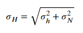
where:
σH = standard deviation of orthometric height
σh = standard deviation of ellipsoidal height
σN = standard deviation of geoidal height
Note: Sample calculations of orthometric height error are included in Appendix F.
Field observations
Length of observation session
When precise ellipsoidal or orthometric heights are required in a network, common session observation times must be increased for these components of the network, as follows:
- KEY Network station observation time must be increased by 15 minutes (resulting in a minimum of 60 minutes common session observation time
- Project Network station observation time must be increased by 15 minutes (resulting in a minimum of 45 minutes common session observation time
Independence of observations
Observations (or occupations) can only be considered truly independent if they do not occur in consecutive sessions. Ideally the re-occupation of a station should occur on another day. If a station must be re-occupied on the same day, there must be a minimum of 2 hours separation in time between the end of the first session and the start of the second.
For any GNSS network that requires precise ellipsoidal or orthometric heights, fully independent/repeat occupations are required for all stations in the project network as defined above.
Additional recommendations
- Fixed height tripods should be used when accurate orthometric/ellipsoidal heights are being determined
- Choke ring antennas should be used in areas where multipath is highly prevalent (for example, downtown urban core of high-rise buildings)
- Ground truthing or confirmation of observed GNSS derived height is strongly encouraged by comparing derived elevations and elevation differences for station elevations determined through Canadian Geodetic Survey’s Precise Point Positioning (PPP) service
Project deliverables
Reports and returns
The final report for a GNSS GPS survey project must provide all the information necessary to evaluate the satisfactory completion of the project objective. Sufficient information must be provided in the report to enable reprocessing of the raw data, if required. The report items identified below are the minimum requirements for a project. Depending on the instrumentation or methodology used, additional information may be required.
Project description
A short description of the objectives of the project are required, including the general location of the survey and number of stations positioned must be presented.
A detailed description of the project quality control plan and the measures taken to ensure the plan was followed must be included.
A description of any problems encountered, and how they were resolved, must be given.
A final network diagram showing all stations occupied must be submitted. It shall be to scale and must show:
- all existing control stations in the project area
- all new control stations
- the baselines observed, complete with session identification
- all repeat baselines
Survey procedures
The returns submitted must be accompanied by a clear description of the survey procedures used in the field. The following information must be provided:
- a summary of the equipment used
- information related to specific procedures used in the field such as values and methods necessary to convert antenna height measurement to vertical height from marker to phase centre
- a summary indicating for each session the stations occupied, their respective start and end time of data collection, and raw data file names
GNSS data processing procedures
A detailed description of the procedures used for processing and verifying the GNSS data in the field or office must be presented. The following information must be provided:
- computer software (version number and date) used in the data processing
- a detailed description of the processing controls and options used
- a description of the ephemerides used their source and datum
- a list of the fixed stations used for coordinate seeding during processing
- information and explanations about data editing performed
- the ionospheric and tropospheric models used
- information and evaluation of the differences between repeat baselines
Adjustment procedures and analysis
A detailed description of the procedures used for adjustment and analysis of the network must be presented. The following information is required:
- computer software (version number and date) used in the adjustment
- the value used for scaling the covariance matrix in the minimally constrained adjustment to account for overly optimistic error estimates
- a justification for any baselines rejected
- an analysis of the residuals, residual outliers and semi-major axes of the 2-D and 1-D 95% relative confidence rejoins between all connected stations from the minimally constrained adjustment
- an analysis of the accuracy, compatibility, and reliability of the existing control
- an analysis of the residuals, residual outliers and semi-major axes of 2-D and 1-D 95% relative confidence rejoins between all connected stations from the fully constrained adjustment
- the local and network accuracy classification of the network stations from the constrained adjustment
All digital data must be submitted on reliable storage device such as thumb drive, external drive, or a secure online utility.
The deliverables shall include:
- all original measurement data (raw data) collected during the project, clearly labeled, and described. Data must also be provided in RINEX (Receiver Independent Exchange) Format, Version 2 or later
- all original field notes, field logs, obstruction diagrams and levelling notes
- new monument location sketches for both new and existing monuments (where required) - preferably in GIF or PDF format
- all GNSS baseline solution files in a digital format including an index file which provides the baseline file names and session identifiers for each baseline
- all GNSS baseline solutions from each session must also be grouped together and saved in a separate file for the session using a filename that contains, minimally, the Session_ID (S#) and the Project_ID, for example: S01_WO2020-102.asc, S02_CO27-130.1.asc, Sess-07_Proj2023-001.asc, etc.
- a summary of the baseline solutions in digital (ASCII) format clearly indicating whether the ambiguities have been resolved and an indication of their quality
- minimally constrained and fully constrained adjustment input files in digital format
- minimally constrained and fully constrained adjustment output files in digital format
- minimally constrained and fully constrained adjustment input files (digital) in GeoLab input file format (version 3 or newer)
- final geographic (latitude, longitude orthometric elevation and ellipsoidal height), UTM and MTM coordinates in digital (ASCII) format
- photos (preferably in JPEG or GIF Formats):
- photo 1 - with the camera pointed down (top-down view of the monument), verification of the physical mark showing its identifier (number)
- photo 2 - a horizon view of the general area of the control marker
- photo 3 - (optional) a photo of tripod/instrument setup at the marker's site
- photo 4 - (optional) any significant obstructions that may affect the quality of the GNSS observations at the station to support/clarify the station's obstruction diagram
- the final report
Appendices
Appendix A – Monumentation
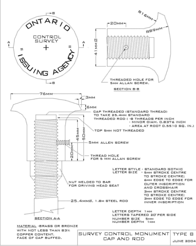
- First image is a top-down view of cap which shows cross section A-A going from left to right and cross section B-B going from top to bottom. Inscription shown on top of cap shows the name “Ontario” curving along the upper edge and “issuing agency” curving along the lower edge. The words “control survey” with a cross below is shown at the centre of the cap.
- Image of cross section A-A shows the top of the cap being 76 millimetres in diameter with a 3 millimetres wide and 6 millimetres tall, angled shoulder. Cap is shown attached to a 25.4 millimetre diameter steel rod with a nut welded to bar for driving head seat below cap. Thread hole is 50 millimetres in height with 45 millimetres of thread, top 5 millimetres not threaded. Cap is threaded with standard thread to take a 25.4 millimetre standard threaded rod with 8 threads per inch, minor diameter of 0.8376 inches and area at root 0.5510 square inches. Threaded hole for 5 millimetre Allan screw and 5 millimetre Allan screw shown 20 millimetres above base of cap.
- Image of cross section B-B shows the base of the cap being 41 millimetres in diameter. Below the shoulder of the cap it has a 16 millimetres radius curve and the top is curved with an 89 millimetres radius. Threaded hole for 5 millimetres Allan screw shown 20 millimetres from base of cap.
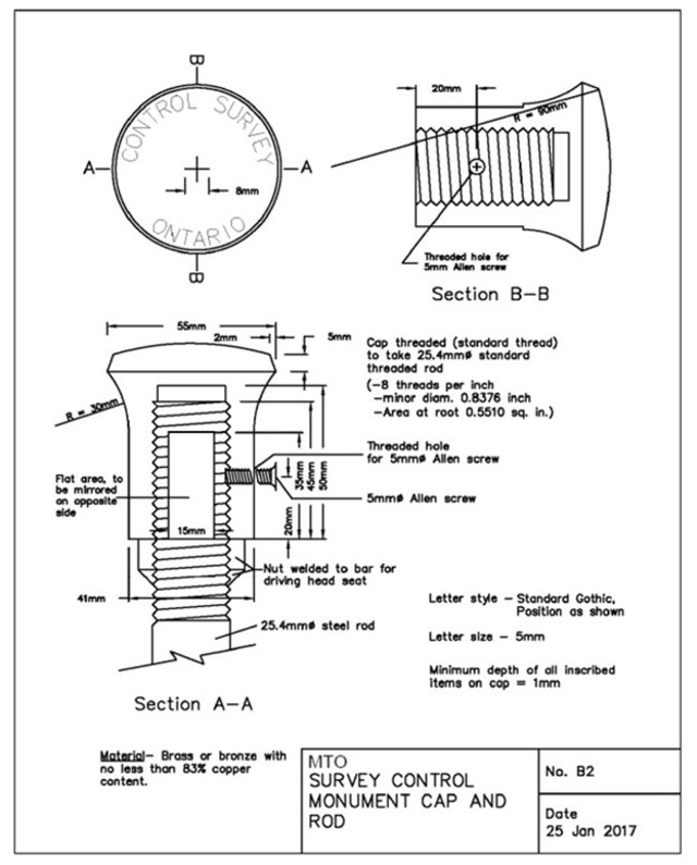
- First image is a top down view of cap which shows cross section A-A going from left to right and cross section B-B going from top to bottom. Inscription shown on top of cap shows the words “control survey” curving along the upper edge and the word “Ontario” curving along the lower edge. An 8 millimetre wide cross is shown at the centre of the cap.
- Image of cross section A-A shows the top of the cap being 55 millimetres in diameter with a 2 millimetres wide and 5 millimetres tall, angled shoulder. Cap is shown attached to a 25.4 millimetre diameter steel rod with a nut welded to bar for driving head seat below cap. Thread hole is 50 millimetres in height with 45 millimetres of thread, top 5 millimetres not threaded. Flat area shown on side being 15 millimetres wide and 35 millimetres tall and is mirrored on opposite side. Cap is threaded with standard thread to take 25.4 millimetre standard threaded rod with 8 threads per inch, minor diameter 0.8376 inch, and area at root 0.5510 square inch. Threaded hole for 5 millimetre Allan screw and 5 millimetre Allan screw shown 20 millimetre above base of cap. Base of cap is 41 millimetres in diameter and below shoulder shows radius of 30 millimetres.
- Image of cross section B-B shows the top is curved with a 90 millimetre radius. Threaded hole for 5 millimetre Allan screw shown 20 millimetres from base of cap.
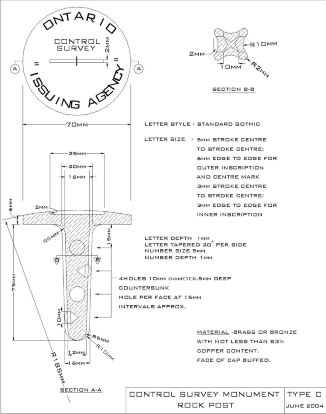
- First image is a top down view of cap which shows cross section A-A going from left to right. Inscription shown on top of cap shows the word “Ontario” curving along the upper edge and “issuing agency” curving along the lower edge. The words “control survey” with a 2 millimetre wide horizontal slot below is shown at the centre of the cap. Cap is shown to have a diameter of 70 millimetres.
- Cross section A-A shows top of cap having a radius of 185 millimetres on it’s face and 6 millimeters thick at edge. 2 millimetre wide slot shown to be 35 millimetres in length. Base tapers from outer width of 20 millimetres, inner width of 16 millimetres to 16 millimetres outer width, 12 millimetres inner width. Bottom point has a radius of 10 millimetres. 4 countersunk holes per face 10 millimetres in diameter and 5 millimetres deep at 15 millimetre intervals approximately.
- Section B-B shown left to right looking down at centre. Section B-B shows an X shaped base with 10 millimetre radius on inside and 2 millimetre radius on outer points. Faces are 10 millimetres apart.
Appendix B - Monument position sketch
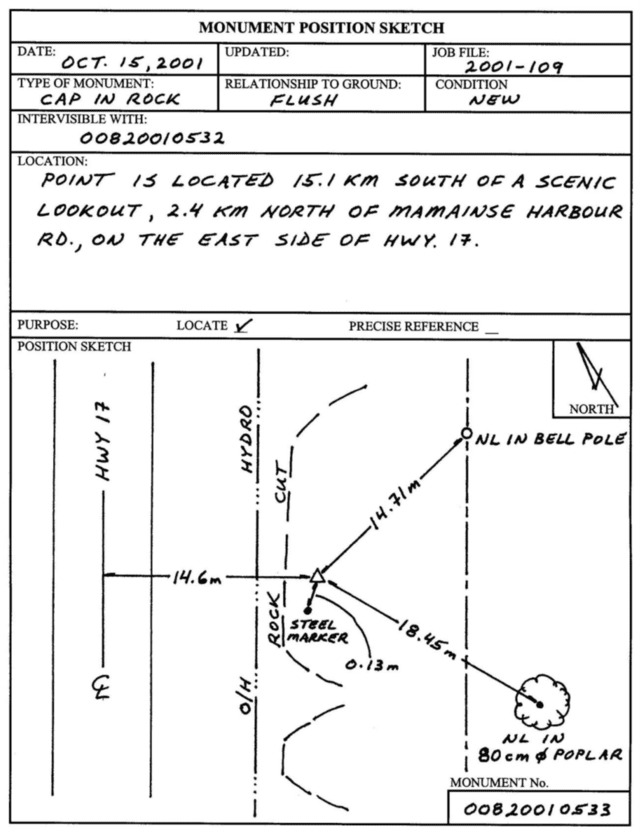
- date: October 15, 2001
- job file: 2001-109
- type of monument: cap in rock
- relationship in ground: flush
- condition: new
- intervisible with: 00820010532
- location: point is located 15.1 kilometres south of a scenic lookout, 2.4 kilometres north of Mamainse Harbour Road, on the east side of Highway 17
- locate: yes
- position sketch: the example shows Highway 17 and the centreline with a measurement of 14.6 metres from centreline to the station. Shows an overhead hydro line and a rock cut. Shows a steel marker 0.13 metres south of station, nail in 80 centimetre diameter polar 18.45 metres southeast of station, and a nail in a bell pole 14.71 metres northeast of station. North arrow is shown in top right corner
- monument number with sample being 00820010533
Appendix C – Network design

Appendix D – Field log sheet
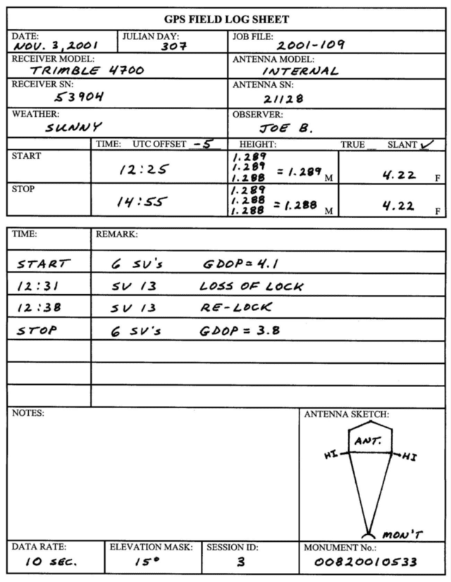
- Title: GPS Field Log Sheet
- Date: November 3, 2001
- Julian Day: 307
- Job file: 2001-109
- Receiver model: Trimble 4700
- Antenna model: internal
- Receive SN: 53904
- Antenna SN: 21128
- Weather: sunny
- Observer: Joe B.
- Start time: 12:25
- Start height: 1.289 metres
- Start slant: 4.22 feet
- Stop time : 14:55.
- Stop height 1.288 metres
- Stop slant: 4.22 feet
- Time: Start - Remark: 6 SV's, GDOP=4.1
- Time: 12:31 - Remark: SV 13 , Loss of lock
- Time: 12:39 - SV 13 - Remark: Re-lock
- Stop: 6 SV's - Remark: GDOP = 3.8
- Date range: 10 sec.
- Elevation mark: 15 degrees
- Session ID: 3
- Monument number: 008200105533
Also included in the example are designated areas for notes and for an antenna sketch.
Appendix E – Obstruction diagram
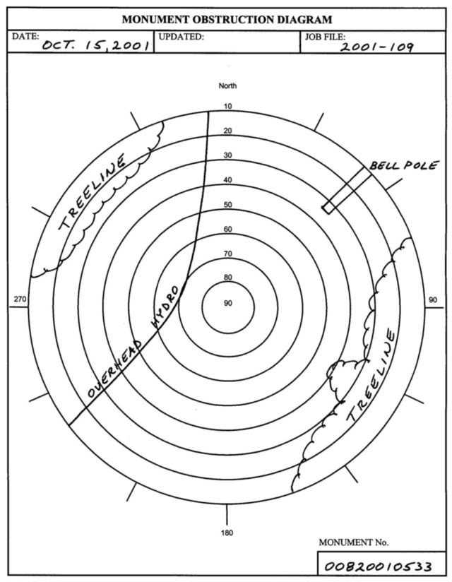
- The diagram features 8 circles expanding out from one center circle. These circles represent 10-degree angles above the horizon. The center circle of the diagram is 90 degrees. As the circle get further away from the center circle, they decrease in angle by 10 degrees. The outermost circle in the diagram is 10 degrees.
- The top of the diagram is labelled as north.
- The east side of the diagram is labelled as 90 degrees.
- The south side of the diagram is labelled as 180 degrees.
- The west side of the diagram is labelled as 270 degrees.
- Sample data in this diagram shows the northwest section of the diagram having a scalloped line representing a treeline.
- In the diagram there is also a curved line running from north to southwest. This line represents an overhead hydro line.
- In the northeast a rectangle extends towards the center. This represents a Bell poll.
- Another scalloped line in the southeast section of the diagram shows another tree line.
- The bottom right portion of the diagram page has a space for a monument number. This diagram’s monument number is 00820010533.
Appendix F – Sample orthometric height accuracy calculationfootnote 2
σh: Ellipsoidal height STD (cm)
1 cm
σN: Geoidal height STD (cm)
1.5 cm
σH: Orthometric height STD (cm)

σh: Ellipsoidal height STD (cm)
2 cm
σN: Geoidal height STD (cm)
1.5 cm
σH: Orthometric height STD (cm)

σh: Ellipsoidal height STD (cm)
3
σN: Geoidal height STD (cm)
1.5 cm
σH: Orthometric height STD (cm)

σh: Ellipsoidal height STD (cm)
5
σN: Geoidal height STD (cm)
1.5 cm
σH: Orthometric height STD (cm)

σh: Ellipsoidal height STD (cm)
10
σN: Geoidal height STD (cm)
1.5 cm
σH: Orthometric height STD (cm)

Footnotes
- footnote[1] Back to paragraph Note: intervisible station pairs are set for azimuth control for conventional survey work
- footnote[2] Back to paragraph The Appendix F table shows standard (1 Sigma) accuracy calculations. To determine 95% confidence values, the results computed above must be multiplied by a factor of 1.96.