Technical bulletin: Using Combined Assessment of Modelled and Monitored (CAMM) results to refine emission-rate estimates
Minimum standards the ministry expects when assessing emission-rate estimates from sources that do not have sufficient data or exceeded the ministry Point of Impingement limit in their initial estimate.
Preamble
The purpose of this Technical Bulletin on “Combined Assessment Of Modelled And Monitored Results (CAMM) As An Emission Rate Refinement Tool” is to provide guidance to persons seeking approval of a proposed CAMM study. This bulletin will set out minimum expected standards that the director will apply in exercising his or her discretion in considering proposed a CAMM results studies on a case-by-case basis. To the extent that this document sets out that something is “required”, “mandatory” or “must” be done, it does so only to identify minimum expected standards, the application of which remain subject to the discretion of the director.
The requirements of this bulletin are compulsory to the extent that they are contained in (e.g. conditions of an Environmental Compliance Approval (ECA) issued under section under section 20.2 of Part II.1 of the EPA or other legally binding instrument). While every effort has been made to ensure the accuracy of the information contained in this bulletin, it should not be construed as legal advice. In the event of a conflict with requirements identified in the regulation, then the regulatory requirements shall determine the appropriate approach.
Introduction
Ontario Regulation 419/05 Air Pollution – Local Air Quality (the regulation) works within the province’s air management framework by regulating air contaminants released into communities by various sources, including local industrial and commercial facilities.
The regulation includes three compliance approaches for industry to demonstrate environmental performance, and make improvements when required. Industry can meet an air standard, request and meet a site-specific air standard or register and meet the requirements under a technical standard (if available). All three approaches are allowable under the regulation.
Provincial air standards are used to assess a facility’s individual contribution of a contaminant to air. They are set based solely on science and may not be achievable by a facility or a sector due to unique technical or economic limitations. In these cases, industries or sectors look to technology and best practices to improve their environmental performance and comply with the regulation.
The regulation places limits on the concentration of contaminants in the natural environment that are caused by emissions from a facility. The concentrations in the natural environment are calculated at a location referred to as a “point of impingement” (POI) which is defined in section 2 of the regulation, as follows:
2. (1) A reference in this regulation to a point of impingement with respect to the discharge of a contaminant does not include any point that is located on the same property as the source of contaminant.
(2) Despite subsection (1), a reference in this regulation to a point of impingement with respect to the discharge of a contaminant includes a point that is located on the same property as the source of contaminant, if that point is located on,
- a child care facility
- a structure, if the primary purpose of the property on which the structure is located, and of the structure, is to serve as,
- a health care facility
- a senior citizens’ residence or long-term care facility
- an educational facility
The Regulation requires that where a facility discharges a contaminant into the air from one or more sources, the concentration at any POI resulting from that combined discharge must be less than the standard prescribed in the regulation. The Ontario Ministry of the Environment and Climate Change (ministry) also uses a broader list of point of impingement limits (ministry POI limits)
Modelling and monitoring are both tools that are used to determine concentrations of specific contaminants in air and both are affected by meteorological conditions as well as the amount of the contaminant being discharged. When modelling and monitoring data are used together, the result can be a more accurate or refined emission rate(s) for a source(s) of contaminant. The use of a CAMM study to refine emission rates is a requirement of the regulation. This is outlined in sections 10, 11 and 12 of the regulation. Section 11 describes the regulatory requirements for the determination of emission rates. In particular, paragraph 3 of section 11 (1) refers to a methodology for determining emission rates using a combination of modelling and monitoring, as follows:
11. (1) An approved dispersion model that is used for the purposes of this Part shall be used with an emission rate that is determined in one of the following ways for each source of contaminant and for each averaging period applicable to the relevant contaminant under section 19 or 20, whichever is applicable:
- the emission rate that, for the relevant averaging period, is at least as high as the maximum emission rate that the source of contaminant is reasonably capable of for the relevant contaminant
- the emission rate that, for the relevant averaging period, is derived from site-specific testing of the source of contaminant that meets all of the following criteria:
- the testing must be conducted comprehensively across a full range of operating conditions
- the testing must be conducted according to a plan approved by the Director as likely to provide an accurate reflection of emissions
- the Director must be given written notice at least 15 days before the testing and representatives of the MOE must be given an opportunity to witness the testing
- the Director must approve the results of the testing as an accurate reflection of emissions
- the emission rate that, for the relevant averaging period, is derived from a combination of a method that complies with paragraph 1 or 2 and ambient monitoring, according to a plan approved by the Director as likely to provide an accurate reflection of emissions
In general, CAMM studies are undertaken to: (a) develop emission rate estimates for sources that have insufficient or low quality emission estimation data available (e.g., sources with fugitive
Although there are many different uses and applications of CAMM assessments, the focus of this technical bulletin is to provide guidance on its use as a potential emission rate refinement tool as required by paragraph 3 of s. 11(1) of the regulation.
Proposed approaches and guidance
Comparisons of modelled results with monitoring data must be done with caution. Model output concentrations depend on emission rates, source parameters and meteorology as well as the accuracy of the dispersion model. The period of available monitoring data and the locations of the monitors are also important factors when comparing modelled results with monitoring data. When used as an emission rate refinement tool, monitoring data should only be compared to modelled concentrations using meteorological data from the same time period (e.g. ambient measurements collected from May to September should only be compared to modelled results using meteorology from the same period).
Monitoring results can be used to identify systemic biases (“biases”) in modeled concentrations, which can occur due to a number of factors including: (a) the adequacy of the surface characteristics, source parameters and building information used in the modelling assessment; and (b) any uncertainties or omissions in the facility’s emission data. Modelling results can also be used to provide information on locating monitoring sites and identifying regions of elevated contaminant concentrations. It is acknowledged that the CAMM methodology outlined in this bulletin may not apply to all fugitive emissions or may become onerous relative to the benefits of refining the emission rate data and that other assessment tools and methodologies may be more appropriate to obtain an accurate reflection of emissions from these sources. For example, the CAMM methodology outlined in this bulletin would not be recommended for sources of emission that have complex building geometries and/or significant downwash effects for which the algorithms of widely available dispersion models are regarded as having reduced accuracy in modelling concentration levels at near-field locations (i.e. within 1 km).
In the above-mentioned cases (and potentially others) it may be more appropriate for the proponent to use other modelling-and-monitoring assessment tools to satisfy paragraph 3 of subsection 11(1) or other methods that would satisfy paragraph 2 of subsection 11(1) of the regulation. In any case, these assessment approaches must be approved by the ministry and proponents are encouraged to consult with the ministry during the pre-assessment plan (“Plan”) development stage. Appendix B discusses the outcomes from a ministry review of methods to measure fugitive emissions.
The accuracy and precision of all components contributing to concentrations of contaminants in air must be respected and considered. The goal is to produce a consistent picture of the situation in order to properly evaluate impacts.
2.1 Pre-assessment plan
In order to be accepted by the ministry, all CAMM must be completed according to a pre-approved Plan. The latest version of form 6323e entitled Request for Approval under paragraph 3 of s. 11(1) of Regulation 419 of a Plan for Combined Analysis of Modelled and Monitoring Results can be found on the ministry website, and is to be submitted to the ministry along with the Plan. Pre-consultation with the ministry is recommended during the development and prior to the submission of the Plan.
The Plan should outline the objectives of the CAMM and describe the methodology in sufficient detail to demonstrate that the objectives will be met. At a minimum, a Plan should include the following elements:
- a scaled site plan that includes the property boundary, building locations, and the location of relevant sources of contaminant
- meteorological information (including the data set to be used, applicable wind roses and local land use information)
- a map of proposed monitoring locations (Note: if mobile monitors are being considered, the approach should be based on wind direction and outlined in detail)
- details of the proposed sampling approach (including the target contaminants, the method to be used, sample frequency and duration, the proposed length of the monitoring program, and laboratory/analytical details)
- the proposed data analysis/screening approach (e.g. how to discern between valid and invalid samples)
- the proposed air dispersion modelling approach (e.g. the model to be used for emission rate refinement, initial target sources for emission rate adjustment, use of any non-regulatory settings in the modelling analysis, etc.)
In general, the proposed monitoring program must satisfy the requirements outlined in the latest version of the Operations Manual for Air Quality Monitoring in Ontario, which contains guidance on ambient monitoring, such as monitoring techniques, locating criteria and other related issues. Proponents wishing to use data collected in a manner that deviates from this guidance are encouraged to discuss this early in the consultation process with the ministry. A sample Plan outline is provided in Appendix A. Appendix B provides additional guidance for the development of a Plan and consultation with the ministry.
After initial approval, any subsequent revisions to the Plan must be submitted and accepted by the ministry. Consultation with the ministry through the development of any Plan revisions is recommended to facilitate ministry consideration and acceptance of the proposed changes.
2.2 Monitoring approaches
This method gives regard to data generated from two types of monitoring approaches:
- long-term fixed-location monitoring stations (also known as “ambient air quality stations”) and
- short-term monitoring.
Long-term fixed-location monitoring stations are generally located to measure airborne contaminant levels in communities that have one or more industrial facilities impacting local air quality.
Short-term monitoring programs are generally focused on developing data for CAMM studies and consist of:
- mobile monitoring where the location of monitoring is potentially variable for each sampling event; or
- temporary fixed-location monitoring stations that are set-up solely to collect data for the duration of the CAMM study.
2.2.1 Long-term fixd location monitoring (Ambient Air Quality Station)
Long-term fixed-location monitors are typically operated year-over-year and can provide a significant quantity of data points to be considered for analysis. A review of long-term fixed-location monitoring data can provide proponents with useful information to potentially refine emission rate estimates and assess the representativeness of refined emission rate values.
2.2.1.1 Analysis of data for long-term fixed-location monitoring
The analysis of long-term fixed-location data typically begins at the local level with the analysis of data from a monitor(s) located in the vicinity the facility and a source(s) of interest. The first step in the analysis is to determine if the ambient air quality station(s) has captured the source(s) of interest by examining the data for general trends that can be linked to the source(s) of interest. The data should be screened based on the wind directions that occurred during each sample. High measured values that occur when the monitor was upwind of the source(s) of interest may indicate additional sources in the area or a meteorological anomaly between the meteorological tower site and the facility where the source(s) is located. These data should be carefully examined to determine how they may be used in the analysis.
Pollution rose analyses of monitoring data can help support the link between the monitoring results and the suspected source(s) of interest. Where multiple monitoring stations are located close to the source of interest, the analysis becomes even more valuable. The wind rose should clearly point towards the suspected source(s); otherwise this may indicate the presence of other unaccounted for sources. Measured levels at or below normal ambient levels may indicate that the source of interest is emitting very little of those specific contaminants; however, the potential for a poorly located monitor (e.g. one that is too far away from the source(s)) should also be considered.
Monitors capturing multiple contaminants that are emitted by the source(s) of interest can also provide useful information. The inclusion of multiple contaminants in the study will allow for a ratio analysis, which has utility in separating different contributing sources at a facility. For example, at some facilities, the ratios of specific contaminants are different when released from stack sources as opposed to sources of fugitive emissions. For contaminants emitted from similar sources at a facility, the contaminant ratios in the emission rates should be similar to the ratios of the measured concentrations. If the measured ratios are not comparable to any of the emission rate ratios this could indicate that unknown sources are contributing, or that there is an error in the emission rate ratios. In these instances, the emission rate estimates and source characteristics should be carefully reviewed.
2.2.1.2 Emission rate refinement using long-term fixed-location monitoring data
The ministry’s experience is that the refinement of emission rate estimates for a specific source(s) of interest using data from ambient air quality stations is often challenging primarily due to the distance that the monitor is located from the source(s) of interest. Most ambient air quality stations have been located to measure representative air quality levels in the communities surrounding industrial facilities and as such are not positioned to capture a specific source(s) of emission. For monitors located greater than 1 km from the source(s) of interest, it’s recommended that this data only be used to assess the representativeness of the refined emission rate estimates rather than to refine emission estimates for the source(s) of interest (see Appendix B for further discussion).
In cases where emission rate refinement using data from long-term fixed-location monitors is determined to be appropriate, the study should not be limited to only the highest measured concentration which may have biases of its own. The concentration values selected for the analysis (i.e. the “hits”) should be greater than measured upwind (i.e. background) concentrations by at least 50%. In cases where known upwind sources of the same contaminant are prevalent it may be appropriate to select hits that are greater than the measured up wind concentrations by at least 200%.
To account for capturing the source(s) of interest and variability in wind direction; the monitor is to be downwind of the source(s) of interest for at least 25% of monitoring period. For example, for an 8-hour monitoring period, the monitor would have to be downwind for a minimum of two hours for a sample to be considered a hit.
The first step in the analysis of data from a long-term fixed-location monitor is to make a selection of hit measurements over the time period for which both modelling and monitoring data are available. For clarity, the monitoring period is determined by the sampling and analytical methods for the specific contaminant being measured and is independent of the averaging time of the standard. The model is then run for a period that matches the monitoring period. For example, if a monitor measured a 12-hr sample, the CAMM analysis would use a dispersion model to predict a concentration averaged over the same period of time that the sample was collected (i.e. 12 hours). The modelled and measured concentration would then be compared.
The ministry generally expects that studies use a minimum of 30 hits for monitoring periods that are greater than 12 hours (i.e. daytime or daily measurements). Studies that use shorter monitoring periods (e.g. 1-hour monitoring periods) should also require approximately 30 hits and these hits are to be collected over at least 20 different days.
The minimum number of hits may vary as a result of: challenges in locating monitors in the prevailing wind directions; having unexpectedly low monitored concentrations; or identifying a large number of confounding sources of air emission. Therefore, the minimum number of hits may vary based upon site-specific conditions and based upon consultation with the ministry during the Plan development stage or after commencement of the monitoring program.
It should also be noted that values measured on calm days might be difficult to model. The meteorological data may show a fairly constant direction at 1 m/s when in actuality the wind was varying in direction and lower in speed. To mitigate for this effect, potential hits are recommended to be screened and only included in the analysis if the wind speeds exceeded 1 m/s for the entire monitoring period and exceeded 2 m/s for at least 75% of the monitoring period. If a proponent needs to deviate from these wind speed screening criteria, the proponent should discuss the circumstances with the ministry and outline the proposed deviation in the submitted Plan.
It is recommended that a site plan plot be set up for each hit measurement. An example site plan plot is provided in Figure 1. This plot should illustrate:
- the ambient measurements for each monitor in relation to the key sources of air emission
- the property-line
- the wind rose for the specific monitoring period/day
- a north arrow, scale
- comments/notes on the source operation for the monitoring period
2.2.2 Variable-location monitoring and short-term fixed-location monitors
For mobile monitors and temporary short-term monitors (i.e. a fixed station that is established for the duration of the refinement assessment), there is usually much less data available for analysis in comparison to the ambient air quality stations. This is because there are a limited number of samples gathered during a limited period of time. However, these monitoring programs are usually designed such that the samples specifically capture air emissions from the target source(s) as samples are generally collected when the monitor is downwind of the source(s) of interest. The goal of designing the monitoring program in this manner is:
- to be able to assess the degree of bias between the modelled and monitored results and
- to refine emission rate estimates, as necessary, for the source(s) of interest.
2.2.2.1 Monitoring data analysis & screening for variable-location monitoring
Similar to the approach set out for the fixed-location monitoring data, the dataset for variable-location monitoring should be subject to a pre-screening analysis to confirm it is linked to the suspected source(s) and that an unbiased downwind measurement (signal) of the source(s) is present as compared to upwind values or normal ambient values. As described earlier, the ratio of the concentration of the contaminant of interest from the source compared to other contaminants emitted by the same source can also be used to help separate different sources or source types. Refer to Chapter 2.2.1.1 for further details.
The analysis for variable-location monitoring data is virtually identical to analyses for the fixed-location monitoring data (see Chapters 2.2.1.1 and 2.2.1.2). In the case of mobile datasets, all downwind samples considered to be a hit will be included in the analysis except where there are known suspect values. Suspect data could be due to inconsistencies in the source(s) operating conditions (e.g. not operating at typical levels) and can be noted as such in the assessment report submitted to the ministry.
To accommodate site or staffing requirements, it may be acceptable for mobile monitoring to be conducted during daytime hours and for varying durations whereas the sources of interest may operate for the entire day. Consideration of the sampling duration must be considered in modelled and monitored data comparison.
Although mobile monitors attempt to take measurements as close to the plume centreline as possible, the wind direction will often shift during the sampling period. If there were changes in wind direction over the sample collection period, the percentage of time that the monitor was downwind must be considered in determining whether the measurement is considered a hit. In general, the mobile monitor should be downwind of the source for 50 to 75% of the monitoring period. For example, for an 8 hour monitoring period, the monitor would have to be downwind for a minimum of 4 hours to be considered a hit.
2.3 Air dispersion modelling approaches
The general approach used in the air dispersion modelling part of the assessment is similar for both fixed and mobile monitors.
When the CAMM is undertaken to refine emission rates, the modelling is usually completed in an iterative process, focusing particularly on sources where there is a high degree of uncertainty in the emission rates. Comparisons between modelled and measured concentrations are done using quantile:quantile (Q:Q) plots and potentially other statistical measures to assess how well the measured concentrations match the modelled results. This is discussed in further detail in Chapter 3.0.
When completing dispersion modelling for a CAMM, care should be taken in determining the model inputs and settings as accurately as possible. The emission rates used in the model must be representative of the actual process/production conditions that occurred during the monitoring period, and will not necessarily reflect the worst case maximum emission rates that the source is capable of. If appropriate, all significant uncertainties related to model inputs should be recorded and subjected to a sensitivity analysis. For example, if there is uncertainty in the height of the buildings causing plume downwash, a second model run using a different building height could show the sensitivity of the modelled results to that parameter.
In order to reduce the impacts of discrepancies between the actual wind directions transporting the source air emissions and the wind directions in the meteorological data set, modelled results for both the fixed and mobile stations are to be output on an arc transcribed through the monitor location. An arc extending 10° on either side of a line extending from the centre of the most significant source to the monitor location should be set up with a total of eleven receptor points; five points equally spaced on either side of the monitor with a single point at the monitor location (see Figure 2). The sampling height of the station should be used as the receptor elevation. The model should be run for the same periods (hours or days) on which valid monitoring data is available.
The use of the most appropriate meteorological data will greatly improve the analysis. The selection of meteorological data should take into account the distance from the meteorological station to the source(s) of interest as well as the proximity to lakes and other local influences (e.g. ridges, mountains, etc.). Shifts in the wind rose between the wind tower site and the facility of as little as 20° could affect comparisons of modelled results with measured concentrations. In addition, appropriate land use characterization could have a significant influence on modelled results.
Biases analyses and emission rate refinement
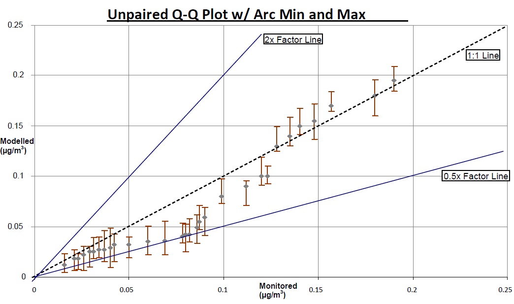
Figure 3 presents a typical example of a bias analysis graph using a Q:Q plot which also includes the maximum and minimum modelled concentration for each hit from the receptors located on the arc. Although the assessment of bias may be presented in different formats, this Technical Bulletin will primarily focus on the use of Q:Q plots and other statistical measures. Alternate approaches proposed by Proponents to check for bias should be reviewed with the ministry and must be articulated in the Plan in order to satisfy the requirements of the Regulation (see Chapter 2.1 and Appendices A and B of this Technical Bulletin on the type of information that should be included in the Plan submitted to the Director).
The Q:Q plot allows rapid identification of biases in favour of modelling or monitoring. The closer the points are to the centre line (1:1 line) the better the correlation between the modelled and monitored data. If data points are consistently above the 1:1 line, this is indicative of a bias towards modelling and may suggest that the estimated emission rates are greater than the actual emission rates occurring for each of the hits. Conversely, data points consistently below the 1:1 line may be indicative of an under estimate of emission rates for each of the hits. Points may lie above or below the 1:1 line as a result of unavoidable variation related to measurement and model fidelity.
Consideration must be given as to whether the data pattern in the Q:Q plot conclusively demonstrates a bias beyond what might be reasonably expected as a result of method uncertainty. To aid in this determination, the Q:Q plot includes reference lines that represent a factor of 2 above and below the 1:1 line. Statistical analysis of the USEPA Prairie Grass model validation dataset has shown that for simple geometries and a near-surface non-buoyant release, CAMM data would generally be expected to fall within the factor of 2 lines. For more complex geometries and source characteristics, less data consistency would be expected.
Any consistent bias beyond levels attributable to method precision should trigger further analysis of the data and modelling inputs, which may include:
- investigation of other contaminants to assist in identifying the source(s) that is contributing to the monitor measurements
footnote 3 - reassessment of source characteristics and emission estimates
- if only a specific monitor is yielding biased results, reassessment of its location in relation to major sources
- evaluation of the validity of meteorological data (e.g. calms, land use, applicability to site)
- consideration of whether the time period used in the model accords with the monitoring period
- assessment of the uncertainty of emission factors or emission rates used as model inputs
3.1 Emission rate refinement procedure
A detailed, step-by-step emission rate refinement procedure is outlined below. An initial unpaired analysis (see Chapter 3.1.2) and any necessary bias analysis/assessment (see Chapter 3.1.3) should be included in the submission to the ministry but any emission rate adjustments (see Chapter 3.1.4) are optional. Table 3.1 summarizes key criteria for the monitoring and modeling analysis and Figure 5 presents a flowchart of this procedure.
3.1.1 Identify hits (mandatory)
Identify hits applying all criteria
3.1.2 Initial unpaired analysis (mandatory)
An unpaired analysis is a mandatory part of a combined modelling and monitoring assessment that will be used to address requirements within the Regulation (i.e. to satisfy the emission rate estimating and refinement requirements of sections 10, 11 and 12 of the Regulation).
Objective: Perform an initial assessment of how well the modelled concentrations match the measured concentrations, and address any potential issues with meteorological anomalies or source characteristics.
- for each monitoring location, rank both the measured and modelled concentrations for the hits from highest to lowest and construct an unpaired Q:Q plot of the modeled concentration at the monitor vs. monitored concentration results (or other alternate approach to assess bias as approved by the Director). For each hit, include range bars
footnote 7 on the graph presenting the maximum and minimum modelled values on the arc (See Figure 3) - examine the plot to identify any biases occurring on the Q:Q plot. A bias would be demonstrated by a majority of the data points on the Q:Q plot occurring above or below the 1:1 line to an extent beyond the expected range of experimental uncertainty
footnote 8 - if the Q:Q plot does not indicate a bias then the assessment is considered complete and the original emission rate estimates for the sources under assessment are considered to be representative of actual emissions. If the Q:Q plot indicates a significant bias, proceed to step 3.1.3.
3.1.3 Bias analysis/assessment
When the Initial Unpaired Analysis demonstrates a bias, one can take the following actions to attempt to resolve the bias.
Source Characteristics:
- verify the source characteristics including building downwash impacts and the release locations of fugitive emissions
- conduct a sensitivity analysis of the source characteristics for the significant source(s) of air emission within realistic parameters (e.g. adjusting the release height for a volume source for cases when this parameter is variable or not well defined)
- further assess source characteristic parameters using data from additional community monitoring stations that are unbiased by other nearby sources of the same contaminants (if available) for measurements collected contemporaneously with the hit measurements
Meteorological Data:
- check the meteorological data for cases with very light wind speeds or inconsistent wind directions. Check whether the land use specified is applicable to the site
- where available, re-evaluate the initial unpaired analysis using meteorological data from a different station(s) (in consultation with and as approved by the ministry under s. 13) located in the vicinity of the facility
Other Contaminant Analysis:
- if applicable, assess the ratio of other contaminants emitted from the same source(s) as the contaminant of interest as described earlier in this bulletin (see Chapter 2.2.1.1)
Initial Emission Rate Estimates:
- confirm that the time period used in the modelling according with the monitoring period
- assess the uncertainty (data quality) of emission factors or emission rates used as model inputs and determine if the level of data quality can be increased
Identify/Confirm Significant Sources:
- review hits paired in space and time to confirm that the model includes the significant sources of the contaminant under assessment. In cases when the modelled results are under-predicting the monitored results, a consistent gap between the modelled and monitored hit data may indicate the presence of a source of the same contaminant that is not included in the model
After completion of some or all of the above analyses, re-perform the modelling analysis for each hit to determine if the bias has been resolved (see Chapter 3.1.1). If the bias is resolved, then the assessment is considered complete and the emission rate estimate(s) for the source(s) under assessment is considered to be representative of the actual air emissions occurring during the assessment. In this case, the submission to the ministry should include a detailed description of how the bias was resolved.
If a significant bias continues to be identified (i.e. the modelled results are consistently under or over the 1:1 line), then an emission rate increase or decrease (as appropriate), for the relevant sources, can be applied which may include considering the ratio of the Robust Highest Concentrations (RHC ) determined for the modelled and monitored datasets (see Chapter 3.1.4).
3.1.4 Emission rate adjustment considering RHC ratios (optional)
The ratio of the modelled and monitored RHC is a preferred statistic
RHC = X{n} + ( [X − X{n}] × ln[(3n − 1) / 2] )
Where:
- n
- is the number of values used to characterize the upper end of the concentration distribution(s). It is suggested that n=10 for assessments of 30 hits; n can be a larger (up to 26) for larger datasets.
- X
- is the average of the n-1 largest values.
- X{n}
- is the nth largest value.
To adjust an emission rate(s) it is suggested that an adjustment factor is developed based on the ratio of the modelled and monitored RHC ’s as set out below:
Factor = (RHCmd / RHCmo)-1
Where:
- RHCmd
- is the RHC determined for the modelled data.
- RHCmo
- is the RHC determined for the monitored data.
The initial emission rate used in the assessment is multiplied by the adjustment factor and the modelling results are reassessed by the steps set out in Chapter 3.1.2. If the reassessment is suitable, then the CAMM assessment is considered complete.
In circumstances where an emission rate adjustment is made, the calculation and comparison of the fractional bias (FB) between the monitored (Mo) and modelled (Md) values (see equation below) both before and after the adjustment is made can be an indicator of the influence of the adjustment on the degree of bias between the modelled and monitored data.
FB = µMo − µMd / 0.5 (µMo + µMd)
Where:
µMo and µMd are the arithmetic averages of the monitored and modelled concentration datasets. An FB that approaches zero is indicative of low average bias between the modelled and monitored data.
Proponents are cautioned that the outcomes of FB are influenced by factors such as the range and skewness of the modelled and monitored datasets. Cases may occur where an adjustment is made and the comparison of the absolute value of the FB ’s calculated before and after the emission rate adjustment increases suggesting that that the adjustment resulted in increased bias between the modelled and monitored data. Although this is not a conclusive signal, in circumstances like this, it is first suggested that proponents consider the applicable steps set out in Chapter 3.1.2 and reassess as set out in Chapter 3.1.2. If this does not satisfactorily resolve the bias, then proponents are encouraged to engage in discussion with the ministry regarding the appropriateness of making an emission rate adjustment.
With respect to the fractional bias statistic there are criteria established by researchers such as Chang and Hanna (2004)
Table 3.1 Summary of Monitoring and Modelling Approaches/Requirements
| Criteria | Fixed-location | Variable-location |
|---|---|---|
| Monitor location relative to facility/source | Downwind for at least 25% of monitoring and operating period | Downwind for at least 50% of the monitoring and operating period |
| Minimum concentration for data validity (“Hit”) |
|
Consider all data, except when suspect. Provide rationale for determining suspect data. |
| Minimum number of hits |
|
|
| Co-contaminant emissions | Measure if possible and do ratio analysis | Measure if possible and do ratio analysis |
| Site specific wind speeds and directions required | Yes, when possible | Yes, when possible |
| Measurements on calm days | “hit” samples be collected for conditions in which wind speeds exceed:
|
Treat with caution – consider in biases plot analysis |
| Site plan plot (see Chapter 2.2.1.1 and Figure 1) | Recommended for each hit | Recommended for each hit |
| Fixed-location | Variable-location | |
|---|---|---|
| Source Emission Rates | Use actual production conditions during monitoring | Use actual production conditions during monitoring |
| Receptor grouping (See Figure 2) | An arc transcribed through the monitor extending 10° on either side of a line originating from the centre of the most significant source to the monitor. | An arc transcribed through the monitor extending 10° on either side of a line originating from the centre of the most significant source to the monitor. |
| Number of receptors per group | Typically 11; one at the monitor location and 5 spaced equidistantly along the arc on either side of the monitor. | Typically 11; one at the monitor and 5 spaced equidistantly along the arc on either side of the monitor. (See Figure 2). |
| Receptor height above ground | Same as height of monitoring station above ground | Same as height of monitoring station above ground |
| Meteorological data | Consult with the ministry’s Environmental Monitoring and Reporting Branch (EMRB ) prior to start of monitoring/modelling assessment | Consult with EMRB prior to start of monitoring/modelling assessment |
| Sensitivity analyses (see Chapter 3.1.2) | As required for significant uncertainties | As required for significant uncertainties |
CAMM Report
In general, CAMM studies are undertaken to: (a) develop emission rate estimates for sources that have insufficient or low quality emission estimation data available; or (b) refine emission rate estimates when initial assessments or monitored results indicate an exceedence of an ministry limit. The maximum emission rate scenario determined through CAMM is also considered in setting a site-specific air standard under the Regulation.
In most cases the above scenarios are undertaken in conjunction with the preparation or updating of Emission Summary and Dispersion Modelling (ESDM) reports. Given the linkage to ESDM reports; proponents can chose to prepare a report documenting the CAMM study either as a separate document submitted with the ESDM or included as an appendix to the ESDM report. Appendix C provides a sample table of contents for this CAMM report.
Figure 1: Example site plan plot
Download Figure 1: Example site plan plot.
Figure 2: Illustration of receptor and monitor arrangement
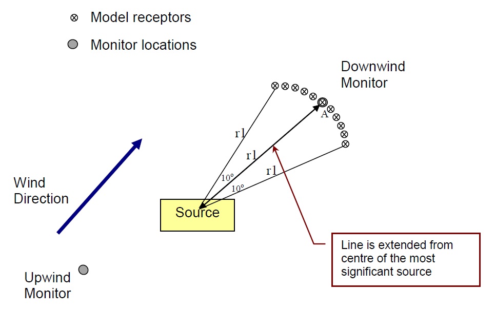
Figure 3: Example Quantile:Quantile (Q:Q) plot
| Hit Days | Production data during sampling period (kg) | Production data during sampling period (tonnes/hr) | Location 1 Monitored Concentration (µg/m3) | Location 1 Monitored Concentration at monitor (µg/m3) | Receptor arc max concentration (µg/m3) | Receptor arc min concentration (µg/m3) |
|---|---|---|---|---|---|---|
| 31-Oct-12 | 4290 | 0.358 | 0.190 | 0.195 | 0.209 | 0.184 |
| 02-Nov-12 | 3990 | 0.333 | 0.180 | 0.180 | 0.196 | 0.160 |
| 05-Nov-12 | 4500 | 0.375 | 0.157 | 0.170 | 0.184 | 0.164 |
| 07-Nov-12 | 4050 | 0.338 | 0.148 | 0.155 | 0.172 | 0.136 |
| 11-Nov-12 | 4020 | 0.335 | 0.140 | 0.150 | 0.168 | 0.141 |
| 12-Nov-12 | 3950 | 0.329 | 0.135 | 0.140 | 0.158 | 0.130 |
| 15-Nov-12 | 4100 | 0.342 | 0.128 | 0.130 | 0.150 | 0.125 |
| 16-Nov-12 | 4158 | 0.347 | 0.123 | 0.100 | 0.110 | 0.092 |
| 20-Nov-12 | 4127 | 0.344 | 0.120 | 0.100 | 0.119 | 0.092 |
Figure 5: Emission rate refinement procedure flowchart
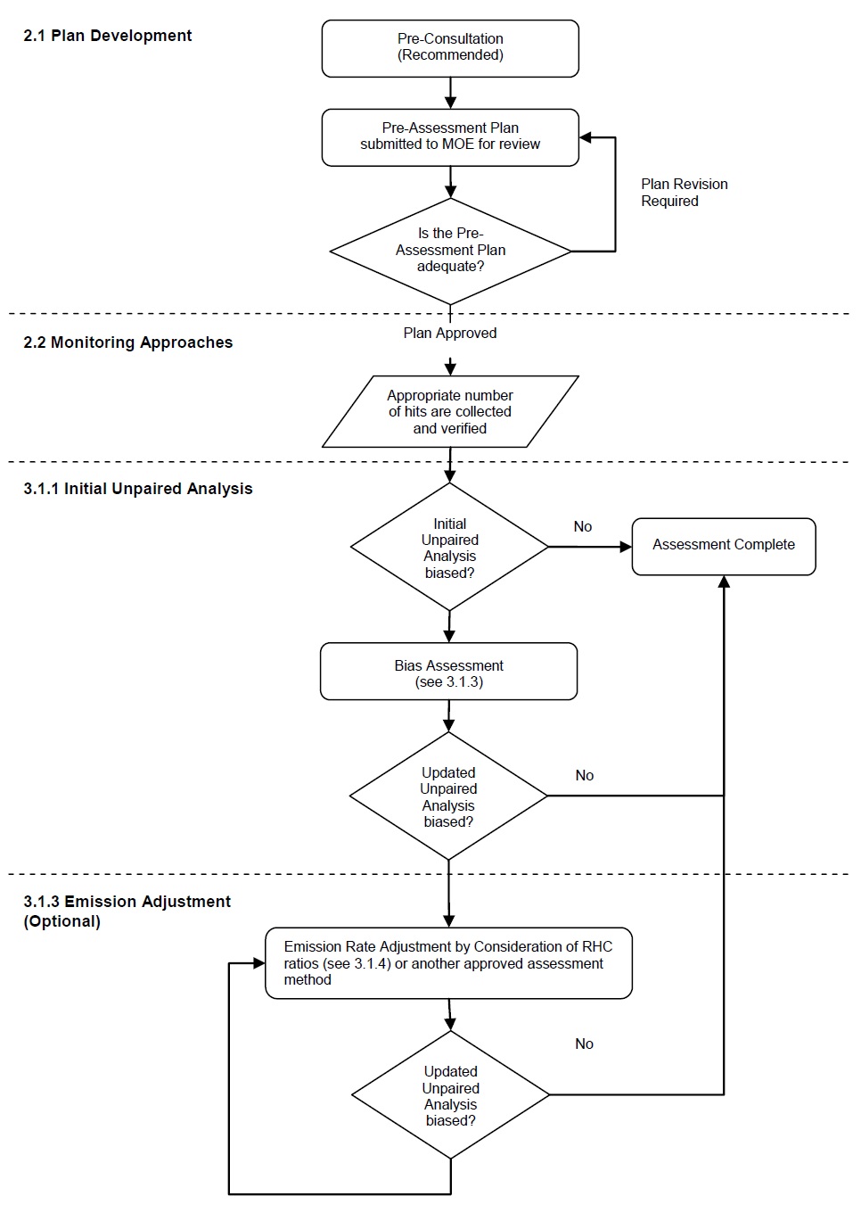
Figure 5: Emission rate refinement procedure flowchart text outline
This figure is a flowchart of the Emission Rate Refinement Procedure. Pre-Consultation with the ministry is recommended, then a Pre-Assessment Plan Is submitted to the ministry for review. If the plan is not adequate then revision is required. Once the plan is approved, then the appropriate number of hits are collected and verified. The initial Unpaired Analysis is then conducted. If the initial Unpaired Analysis is not biased, then the assessment is complete. If the initial Unpaired Analysis is biased, then a Bias Assessment is conducted. If the updated Unpaired Analysis is not biased then the assessment is complete. If the updated Unpaired Analysis is biased, then the Emission Rate can be adjusted by consideration of Robust Highest Concentration ratios or another approved assessment method. If the updated Unpaired Analysis is not biased then the assessment is complete.
Appendix A
Sample Pre-Assessment Plan Outline
- Introduction
- Purpose and objectives of CAMM study
- Facility description
- Process flow diagram
- Scaled site plan
- Including property boundary, building locations, and the location sources of air emission
- Description of significant sources
- Process/Source description
- Identification of contaminants and release points
- Proposed monitoring program
- Proposed monitor locations (including map)
- Meteorological information
- Information regarding the monitoring station, data set to be used, applicable wind roses and local land use information
- Details of the proposed sampling approach
- Sampling equipment, target contaminant(s), sampling and analytical methods, laboratory accreditation(s), sample frequency and duration and the proposed length of the program
- Proposed monitoring data analysis
- Proposed data analysis/screening approach (i.e. how to discern between valid and invalid samples)
- Proposed modelling analysis
- Modelling approach for significant sources
- Land use information, source information, proposed receptor grid
- Receptor information and proposed grid
- Identification of specialized approaches
- Indicate any non-regulatory modelling approaches or special configurations/characterizations for sources
- Modelling approach for significant sources
- Proposed assessment methodology
- Proposed unpaired assessment
- Proposed bias assessment
- Proposed use of Q:Q plots, identification of any additional bias assessment tools
- Schedule
- Outline the overall schedule for the assessment and any factors in scheduling such as seasonal considerations for monitoring
List of figures
None.
List of appendices
Appendix A - Form 6323e “Request for Approval Under paragraph 3 of s.11(1) of Regulation 419 of a Plan for Combined Analysis of Modelled and Monitoring Results.
Appendix B - Request for Approval under s.13(1) of Regulation 419/05 for use of Site Specific Meteorological Data (if applicable).
Appendix B
Additional guidance for the development of a Pre-Assessment plan
The purpose of this Appendix is to provide additional guidance for the development of an acceptable pre-assessment plan (Plan) for a CAMM assessment. The ministry’s experience is that CAMM is most applicable to refining the accuracy of emission rate estimates for sources of contaminant that have fugitive emissions. These types of sources typically cannot be readily source-tested and as such have limited or lower quality emission rate estimation data available.
In order to be accepted by the ministry, CAMM studies must be completed according to a Director approved Plan
Consultation Regarding the CAMM Plan
After determining that refinement of emission rate estimates is required for a source(s) of contaminant, a proponent may wish to contact the ministry to set up a meeting at the proponent’s site to review the emission estimating approach under consideration. Having such a meeting early in the process will increase the likelihood of the CAMM Plan being approved by the Director. Representatives for this meeting may include:
- the proponent and consultant/advisor (as applicable)
- the ministry Area/District/Regional office staff responsible for the facility including Regional Technical Support Staff
- the ministry Environmental Monitoring and Reporting Branch (EMRB )
- the ministry Standards Development Branch (SDB)
- the ministry Environmental Approvals Branch
The purpose of this initial meeting is to set objectives and outline the emission rate refinement assessment approach to a sufficient level of detail such that a Plan can be developed and submitted that is acceptable to the Director. Suggested information to be made available for this meeting should include at a minimum:
- a scaled site plan (including property boundary, building locations, and the location of air emission sources)
- meteorological information (including the data set to be used, applicable wind roses and local land use information)
- information regarding the source(s) of emission including mode of operation (batch vs. continuous), potential for malfunction, potential for variability in production and emission rates
- potential/proposed monitoring locations for the assessment and an indication of whether the monitors will be fixed or mobile
- details of the proposed sampling approach (including the target contaminant(s), method to be used, trigger criteria for sampling events, sample frequency and duration, the proposed length of the monitoring program, and laboratory/analytical details)
- a proposed data analysis/screening approach (e.g. how to discern between valid and invalid samples)
- a proposed air dispersion modelling approach (e.g. model to be used for emission rate refinement, initial target sources for emission rate adjustment, use of any non-regulatory settings in the modelling analysis, etc.)
Outcomes from this initial discussion will provide direction to the proponent in preparing the Plan. The discussion will also assist in estimating the time needed to prepare and submit the Plan to the Director for approval.
Considerations for developing a CAMM plan
The following outlines key aspects to be considered in the development of a Plan:
Location of Monitors: Short-term on-site monitoring stations need to be sited considering: (a) the safety of personnel associated with the monitoring program; (b) the criteria set out in the latest version of the Operations Manual for Air Quality Monitoring in Ontario such as the availability of power and non-interference with operations at the facility. More specifically, monitoring stations are to be sited based upon a number of factors including:
- the proximity to the source(s) of interest – in particular, the monitor must be located close enough to capture emissions from key sources while minimizing potential errors related to near-field source impacts that can affect the accuracy of modelling predictions and measured concentrations
- the prevailing wind directions
- the presence of another possible source(s) discharging the same contaminants in the vicinity of the source(s) that is under assessment
- the height of discharge from the source(s)
Where available, consideration should be given to analyzing existing data from community ambient monitoring stations in the vicinity of the source(s) under assessment provided that these stations are suitably located with respect to the sources. It may prove useful to coordinate the sampling schedule of the short-term refinement study with those collected from the community monitoring station. Pre-consultation with the ministry regarding the use of data from existing ambient monitoring stations is recommended and in general, the ministry will only accept the use of data from stations that are located and operated in accordance with the latest version of the Operations Manual for Air Quality Monitoring in Ontario. Data from coordinated sampling events amongst these monitors can be utilized to assess for potential biases such as a bias due to poor source characterization.
The use of off-property ambient air quality station data for emission rate refinement requires careful consideration by proponents wishing undertake this for a source(s) of contaminant. The experience of the ministry is that the accuracy of emission rate refinement from community monitor data diminishes with distance
Differentiating between sources of the same contaminant: In cases where there is more than one source of the same contaminant at the facility or in the vicinity of the facility; additional measures can be undertaken to:
- measure different size fractions of particulate contaminants in order to distinguish between different sources (e.g., roadway fugitive particulate sizing is often different than fugitive particulates emitted from furnaces and process buildings)
- specify more restrictive wind angle vectors to eliminate the potential contribution from nearby sources of emission. This may impact the ability to obtain the minimum hits required for a CAMM if the wind angles become too restrictive
- measure the ratio of the contaminant(s) of interest to other contaminants emitted by the same source in order to “fingerprint” the source of interest. Provided the monitor has effectively captured the source of interest, then the ratio of the emission rate of the contaminants from the source should be roughly the same as the ratios of the same contaminants measured at the monitoring station. If the measured ratios are not comparable to any of the emission rate ratios this could indicate that several sources are contributing, or that there is an error in the emission rate ratios
- monitor to capture emissions during specific times of the day to take advantage of patterns in process operations or meteorology and potential resulting changes in dispersion characteristics that can assist in differentiating between sources
Cost of Monitoring: The intent is to select methodologies, number of samples and sampling protocols that achieve the objectives of the CAMM program while minimizing costs to the proponent. For example, monitoring for contaminants such as polycyclic aromatic hydrocarbons (PAH’s) are relatively costly to analyze in comparison to other contaminants and thus require careful analysis to ensure the selected samples are verified hits that can be effectively used for the inter-comparison of the modelled and monitored data.
Modelling Considerations: The experience of the ministry is that the accuracy of CAMM is diminished for a source(s) of emission with complex building geometries and significant downwash most likely due to the challenges representing these phenomena accurately within widely available dispersion modelling algorithms. Proponents are encouraged to discuss these considerations with the ministry early in the consultation process to determine if alternate dispersion models not currently approved under the Regulation would mitigate these effects. The use of currently unapproved dispersion models is required to be reviewed and approved under s.7 of the Regulation by the ministry’s EMRB prior use for a CAMM assessment. If these accuracy concerns cannot be addressed adequately through the use of unapproved dispersion models then consideration should be given to assessment tools other than CAMM to obtain an accurate reflection of emissions from the source(s).
Consideration of other methods to refine emission rate estimates
During 2011/2012, the ministry retained a third party consultant to review and analyze emission assessment approaches/methods used in other jurisdictions and to provide recommendations to the ministry regarding Ontario’s CAMM methodology. One of the conclusions from this study is that the CAMM methodology may not apply to all types of fugitive emissions and that other assessment methods which may satisfy paragraph 2 of s.11(1) of the Regulation may be more appropriate to obtain an accurate reflection of emissions. Measurement techniques recommended by the consultant for consideration
- various Optical Remote Sensing (ORS ) techniques
- source testing for non-stack sources
- upwind-downwind assessments
- exposure profiling
Optical remote sensing: Optical Remote Sensing (ORS ) refers to measurement techniques that use light to measure contaminant concentrations and emission rates in the field. ORS is based on using optical instruments to develop a path-average concentration through the plume from one or more sources. Depending on the ORS application, the concentration data can be used for a number of purposes including locating emission sources (hot spots) and mass emission rate determination. To determine the mass emission rate, meteorological data is collected concurrently with the concentration measurements. ORS techniques have been applied to measure fugitive emissions and emissions from flares.
The following documents provide a comprehensive description of the types of techniques, instruments and applications which are collectively referred to as ORS.
- EPA Handbook: Optical Remote Sensing for Measurement and Monitoring of Emissions Flux (December 2011)
- Other Test Method 10 (OTM10) Optical Remote Sensing for Emission Characterization from Non-point Sources (USEPA, 2006)
Examples of optical instruments that can generate path-integrated concentration data include:
- Open-Path Fourier Transform Infrared (OP-FTIR) Spectroscopy
- Ultra-Violet Differential Optical Absorption Spectroscopy (US-DOAS)
- Open-Path Tunable Diode Laser Absorption Spectroscopy (TDLAS)
- Path-Integrated Differential Absorption LIDAR (PI-DIAL)
An advantage of ORS monitoring is that it is capable of measuring emissions from many types of sources.
Potential VOC source resting techniques for non-stack sources: The USEPA document entitled the Protocol for Equipment Leak Emission Estimates
- approach 1 – average emission factor approach
- approach 2 – screening ranges approach
- approach 3 – USEPA correlation approach
- approach 4 – unit-specific correlation approac
With regards to the data quality requirements set out under the Regulation, the application of Approaches 1-3 would not result in an accurate reflection of emissions of the highest data quality given the reliance within the Approaches on emission factors and/or generic correlation equations. Approach 4 may satisfy the Regulation
Another potential example discussed in the consultant study was the techniques utilized by the USEPA in the development of the AP-42 emission factors for coke oven door leaks. The report Final Phase I Method Validation Report for Quantitative Coke Oven Door Leak Measurement Study
Fugitive particulate emission assessment method: The most recent Background Document to AP-42 Section 13.2.1 Paved Roads published in January 2011
Upwind-downwind: The upwind-downwind procedure involves measuring suspended particulate concentrations upwind and downwind of a source of interest. The downwind measurements are recommended to be made at a minimum of two downwind distances and three crosswind locations to characterize the plume. The greater the number of samples, the better the characterization of the plume, including plume spread, centreline location, and plume shape. The upwind measurements constitute the background concentration. The technique involves the subtraction of the background concentration, and then using a dispersion model to back-calculate the source emission rate required to produce the measured concentrations. The upwind-downwind method often assumes a Gaussian plume shape. In a more complex setting, where emissions may have a heterogeneous spatial release pattern, this assumption may lead to poor characterization.
Exposure profiling: This method involves isokinetic sampling downwind of the source(s) of interest. A sampling network designed to cover the cross-section of the plume is employed that also includes vertical monitors. Typically 90% of the plume mass should be covered, which can be estimated based on assumptions of plume distribution. The method then uses a “mass-balance calculation scheme” to estimate the emissions as is employed in typical in-stack isokinetic sampling such as USEPA Method 5. No indirect calculation of the emission rate through the application of a generalized dispersion model is required.
Comparison of CAMM data to long-term fixed-location monitoring results
Although not required by this methodology, some proponents may wish to compare modelled concentrations using the refined emission rate data from CAMM to existing ambient monitoring data in the vicinity of the facility/source if this is available. Proponents wishing to present these types of comparisons to the public are encouraged to consult with the ministry before presenting this information. In making these comparisons, it is recommended that the proponent use an emission rate(s) representative of average operating conditions in the model for comparison to the monitored values, which should be averaged as well. Further, it is also recommended that all monitor data (including zero values) be included in the comparison of the two datasets. Other analyses such percentile comparisons between the modelled and monitored data, may also be useful to understand the representativeness of the modeled concentrations. These comparisons reduce the impacts of outliers in either the monitoring or the modelling results. In instances where there are other sources of the target contaminants, the impact of background sources on measured concentrations may also need to be taken into consideration.
Appendix C
Sample CAMM report table of contents
Executive Summary
- Introduction
- Purpose and objectives of study
- Facility description
- Process flow diagram
- Scaled site plan
- Description of Significant Sources
- Process/Source description
- Identification of contaminants and release points
- Monitoring Data
- Monitor description and locations (including map)
- Meteorological data review
- Overview of meteorological data and comparison to “hit” screening criteria
- Monitoring data review
- Overview of measured results and comparison to “hit” screening criteria
- Summary of monitored hits
- Operating conditions and emission Rate calculations
- Summary of operational data for “hit” events
- Facility/source operational/production data for each hit
- Emission rate calculation summary
- Explanation of methods for emission rate calculations including sample calculations
- Summary of operational data for “hit” events
- Dispersion modelling
- Summary of model inputs
- Identification of specialized approaches
- As applicable, indicate any:
- non-regulatory modelling approaches or special configurations/characterizations for sources
- sensitivity analyses that were conducted with respect to model input parameters
- contaminant ratio analyses undertaken.
- As applicable, indicate any:
- Bias analysis and emission rate refinement
- Initial unpaired assessment
- Include initial unpaired Q:Q plot
- Bias assessment
- Emission rate adjustments (optional)
- Include revised unpaired Q:Q plot
- Initial unpaired assessment
- Findings and conclusions
List of figures
- site plan including monitor locations
- site plan plots and wind roses corresponding to each hit
- Q:Q Plots
List of appendices
- model input file(s)
- as applicable, any Notices issued under the Regulation for the assessment and relevant correspondence from the ministry such as Plan approvals and special guidance regarding modelling parameters.
Footnotes
- footnote[1] Back to paragraph The generic term "limits" in the context of this Technical Bulletin means any numerical concentration limit set by the ministry including standards in the schedules to the Regulation, guideline values and recommended screening levels for chemicals with no standard or guideline value. The ministry Air Contaminants Benchmarks List (ACB List) summarizes standards, guidelines and screening levels used for assessing point of impingement concentrations of air contaminants.
- footnote[2] Back to paragraph The United States Environmental Protection Agency (USEPA) defines fugitive emissions as "those emissions which could not reasonably pass through a stack, chimney, vent or other functionally-equivalent opening"
- footnote[3] Back to paragraph An investigation of other contaminants could include a comparison of the ratios of the concentrations of different contaminants from the monitor measurements with the ratio of concentrations of those contaminants at the source(s) (e.g., within feed material and/or within stack discharges to atmosphere).
- footnote[5] Back to paragraph At this step it is also appropriate to analyze the data with respect to the wind directions for the measurement period to check for inconsistencies with identified air emission sources. High measured concentrations which are not consistent with identified air emission sources could be due to other air emission sources that are at the facility but not properly quantified or included in the modelling assessment. Additional source-specific monitoring could be required to quantify air emissions in this case.
- footnote[6] Back to paragraph Malfunction events are removed from consideration as being hits. For the purposes of this Technical Bulletin a malfunction is considered as an unplanned scenario occurring due to an infrequent failure of a source to operate in a usual manner. The exclusion of a malfunction event should be supported with additional information regarding the cause and frequency of occurrence of the malfunction.
- footnote[7] Back to paragraph The presentation of the maximum and minimum values (range bars) predicted on the arc for each hit can provide insight into potential errors in the modelling and monitoring data. For example, monitor values that are consistently close to the maximum values predicted by the model on the arc can be an indicator that potential errors in wind direction have had a minimal effect.
- footnote[8] Back to paragraph Figure 3 also indicates 0.5× and 2× factor lines which can also aid in assessing the magnitude of the demonstrated bias.
- footnote[9] Back to paragraph Perry, Cimorelli, Paine, Brode, Weil, Venkatram, Wilson, Lee, Peters, AERMOD : A Dispersion Model for Industrial Source Applications. Part II: Model Performance against 17 Field Study Databases, Journal of Applied Meteorology, 26 October 2004, Volume 44, pp. 694-708
- footnote[10] Back to paragraph Chang J., S. Hanna, 2004: Air quality model performance evaluation. Meteor. Atmos. Phys., 87, 167-196.
- footnote[11] Back to paragraph The MOE may consider deviations from the minimum specified number of "hits" based on information provided by the proponent during consultations and included in the submitted assessment Plan.
- footnote[12] Back to paragraph CAMM can also be used to refine source characteristics (rather than emission rates) for non-stack type sources; undertaking a different approach than what is used for emission rate refinement. The approach for source characteristic refinement is generally more complex and labour intensive. Monitors generally have to be placed in very close proximity to the target source(s) and the approach may require multiple monitors per source or source-grouping to provide useful information. The use of tracer gases to minimize uncertainties in emission rates might also be useful.
- footnote[13] Back to paragraph Through assessments undertaken by the MOE , it was found that the exclusion of monitored data based on hit criteria collected at distances of 1 km or greater from a source of interest introduced a bias which was not apparent when all of the monitoring data were included in the analysis.
- footnote[14] Back to paragraph Proponents need to review the applicability of these methods with site-specific considerations
- footnote[15] Back to paragraph United States Environmental Protection Agency, Protocol for Equipment Leak Emission Estimates, EPA-453/R-95-017 (November 1995).
- footnote[16] Back to paragraph Subsection 12(1.1) of the Regulation allows the Director to accept source-testing over a range of operating conditions (paragraph 2 of subsection 11(1)) as the final stage in the refinement process for the emission rate estimates if the Director is of the opinion that the emission rate will be accurately determined.
- footnote[17] Back to paragraph Final Phase I Method Validation Report for Quantitative Coke Oven Door Leak Measurement Study, ENSR Consulting and Engineering, for American Iron and Steel Institute, Washington, DC. December 1991.
- footnote[18] Back to paragraph United States Environmental Protection Agency, Emission Factor Documentation for AP-42, Section 13.2.1 Paved Roads, January 2011.