Appendices

Appendix 1: Sample Pollutant Log

Download Sample Pollutant Log

Appendix 2: List of Activities to be performed during Station Visits

One of the main purposes of monitoring station visits is to verify the proper operation of the monitoring equipment and of data acquisition systems (DAS) to ensure the collection of valid and complete data. A second important purpose is to verify the continued safe and secure environment at the station. Diagnostic tests, which can be performed remotely on various monitoring equipment and station parameters, complement the station visit verification.

Station visits should be documented in the site log. The following is a list of recommended activities to be performed at the station:

• Examine the external station conditions including the inlet probe for damage or blockage. Periodically review the station characteristics for any change or modification to the station to ensure that siting criteria continue to be met.
• Examine the manifold, if applicable, the transfer lines (or inlet line) and the inlet filters for dirt build-up and replace the filter or clean the lines as required. Examine the seals in the sampling system, the scrubbing and drying agents, and replace as required.
• Perform zero and span verifications on the analyzers at least monthly. Record the values and note abnormal deviations. All adjustments need to be documented.
• Perform preventative maintenance as prescribed in the instrumentation operations and maintenance manuals.
• Check the heating/cooling system to ensure that the station temperature is maintained in the required temperature range.
• Ensure that the analyzers are in the sample mode before exiting the shelter.
• Ensure that the shelter door and gate (if applicable) are locked upon leaving the station.

Appendix 3: Guidance for Electronically Submitting Validated Data

The ministry requires electronic submission of raw and edited emitter data on a quarterly basis. This data will then be uploaded into a database. Prior to the first submission of data, the ministry requires that Table 8 be submitted along with a sample of the data to confirm the format in which the data will be received so that the ministry can initialize and test the industry station in the database.

The first column will always contain the date and the second column time. Please be sure that the format of the first two columns is correct and that the date and time have been delimited. It is important that the format be identical each quarter. Data is to be submitted as a time series, not as a monthly matrix. Acceptable data formats include Excel, Comma Separated Values (CSV), or Enview. Each quarter the submission must include a combined file for the three months and the files must contain data ordered from oldest to newest, (e.g., Jan 01/13 0:00 to Mar 31/13 23:59). Examples of acceptable formats are provided in Tables 9 and 10.

If the emitter makes any changes (including service pack installation and upgrades) to their systems after the initial acceptance of their data format by the ministry, the emitter should verify that the formats have not changed. If the data is no longer importable into the ministry’s database, the ministry will provide guidance about the problems and the emitter may be asked to resubmit the data.

Table 8: Station Registration Template

Download Station Registration Template

Table 9: Excel Data Submission

A	B	C	D	E	F	G
Date	Time	TRS	PM2.5	Temp	Wind Speed	Wind Direction
04/01/2006	1:00	−0.031	3.5	0.02	14.4	8
04/01/2006	1:30	−0.026	3.967	−0.148	15.067	4.2
04/01/2006	2:00	0.004	3.8	−0.114	11.467	6.6
04/01/2006	2:30	0.006	3.267	−0.249	10.533	12.9
04/01/2006	3:00	−0.002	6.867	−0.484	9.133	11.3
04/01/2006	3:30	−0.019	1.833	−0.517	5.467	10.4
04/01/2006	4:00	−0.002	5.55	−0.585	3.4	342.8

Table 10: CSV Data Submission

Date,Time,TRS,STEM,TRST
05/29/2007,00:00,1,24,913
05/29/2007,00:30,1,24,913
05/29/2007,01:00,1,23,913
05/29/2007,01:30,No Data,No Data,No Data
05/29/2007,02:00,1,24,913
05/29/2007,02:30,1,23,913
05/29/2007,03:00,1,24,913

Table 11: Sample of Non-Continuous Data Format for Submission

Download Sample of Non-Continuous Data Format for Submission

Appendix 4: Sample Edit Log Table

Table 12: Sample edit log table

Download Sample Edit Log Table

Examples of Acceptable Edit Actions

• Add offset of
• Delete hours
• Zero Correction
• Slope Correction
• Manual data entry for missing, but collected data
• Invalidating span & zero check data
• Invalidating data due to equipment malfunctions and power failures.
• Invalidating data when instrumentation off-line
• Marking data as out-of-range

Appendix 5: Wind Speed and Direction Calculations

The following equations used to calculate wind speed and wind direction values were taken from the US EPA document entitled QA Handbook for Air Pollution Measurement Systems, Vol. IV: Meteorological Measurements, Version 1.0 (Draft) EPA-454/D-06-001, October 2006.

Wind Speed Average Calculation

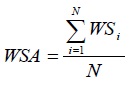
1. Horizontal wind speed (WSA) is scalar horizontal wind speed
2. Horizontal wind speed (WSA) may be averaged into 1-minute, short term (e.g., 5-minute), and 1-hour calculations of mean (scalar) horizontal wind speed.
3. The following is the standard form of the equation used for calculating scalar, or horizontal wind speed (WSA):

   

   where

   WS_i

   instantaneous horizontal wind speed (scalar)

   N

   number of instantaneous samples (typically 1 second)

Horizontal Wind Direction

1. Horizontal wind direction is a circular function with values limited to between 001 and 360 degrees.
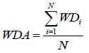
2. The hourly calculation of wind direction mean is a crossover-corrected average of the instantaneous wind direction samples.
3. A crossover algorithm for handling wind direction crossover through north is used that compares the current instantaneous wind direction value to the average of all the preceding wind direction values for the pertinent averaging period. If a difference of more than +180 degrees is found, 360 degrees is subtracted from the current value; or if a difference of less than −180 degrees is found, then 360 degrees is added.
4. The following is the equation used for calculating the mean horizontal wind direction (WDA):

   

   where

   WD_i

   instantaneous horizontal wind direction (scalar)

   N

   number of instantaneous samples

Sigma Theta Calculation

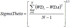
1. Sigma theta calculation is the standard deviation of the horizontal wind direction.
2. The standard deviation of the horizontal wind direction, or sigma theta, is calculated from the instantaneous wind direction samples. An algorithm similar to the crossover algorithm used for horizontal wind direction is used for sigma theta.
3. Sigma theta can be calculated and averaged into 1-minute, short term (e.g., 5-minute), and 1-hour means.
4. It has been suggested that the upper limit of sigma theta should be limited to 103.9 degrees (Yamartino, 1984). The equations used do not impose a limit to the range of possible sigma theta values recorded to eliminate any bias that an upper limit may impose.
5. The following is the form of the equation used for computing sigma theta from horizontal wind direction (WD):

   

   Where

   WDA

   mean horizontal wind direction

   N

   number of instantaneous samples

Vertical Wind Speed Calculation

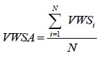
1. Vertical wind speed is the vertical component of wind flow. Vertical wind flow can be positive (upward), or negative (downward).
2. Vertical wind speed (VWSI) can be averaged into 1-minute, short term (e.g., 5-minute), and 1-hour means (VWSA).
3. The following is the form of the equation used for calculating mean vertical wind speed:

   

   where

   VWS_i

   instantaneous vertical wind speed (scalar)

   N

   number of instantaneous samples

Sigma w Calculation

1. Sigma w is standard deviation of the mean vertical wind speed (VWSA).
2. Sigma w can be averaged into 1-minute, short term (e.g., 5-minute), and 1-hour means.
3. The following is the form of the equation used for calculating sigma w:

   

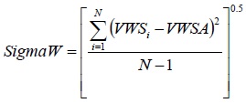
   where

   VWSA

   instantaneous vertical wind speed (scalar)

   N

   number of instantaneous samples

Sigma Phi Calculation

1. Sigma phi is calculated using the Sigma w and horizontal wind speed (WSA) data channels.
2. Sigma phi can be averaged into 1-minute, short term (e.g., 5-minute), and 1-hour means.
3. The following is the form of the equation used for calculating sigma phi:

   

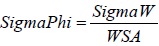
   The above equation yields sigma phi in units of radians and it is converted to degrees using the following equation:

   Sigma phi (degrees) = Sigma phi (radians) * 57.2958

Resultant, or Vector Wind Speed and Direction Calculation

1. The hourly calculation of resultant or vector wind speed and direction provide a vector mean of all of the instantaneous samples of wind direction and wind speed sampled each hour.
2. Sigma phi can be averaged into 1-minute, short term (e.g., 5-minute), and 1-hour averages.
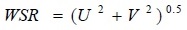
3. The following are the equations used for calculating vector wind speed and vector wind direction:

   

   

   

   

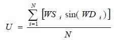
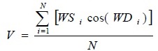
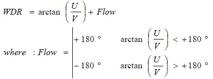
   where

   U

   east-west component of wind

   V

   north-south component of wind

   WDR

   resultant wind direction (vector average)

   WSR

   resultant wind speed (vector average)

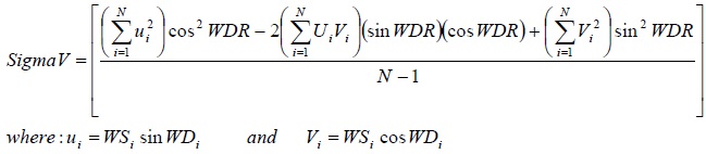
Sigma v Calculation

1. Sigma v is the standard deviation of the instantaneous wind speed normal to the hourly resultant wind direction.
2. Sigma phi can be averaged into 1-minute, short term (e.g., 5-minute), and 1-hour means.
3. The following are the equations used for the calculation of sigma v:

   

Appendix 6: Calculation Procedure for Method Detection Limit (MDL)

This appendix has been reproduced from the original MOECC guidance document Estimation of Analytical Method Detection Limits, originally published in 1988 and revised in 1991.

Introduction and Background

The Method Detection Limit (MDL) is a statistically defined decision point such that measured results falling at or above this point are interpreted to indicate the presence of analyte in the sample with a specified probability, and assumes that there are no known sources of error in identification or biases in measurement.

For the purposes of this protocol, the MDL is defined as having a confidence limit of 99%. This confidence limit defines the multiplication factor used from Student’s t-tables relating MDL to the analytical precision. This Student’s t-value depends on the amount of data used to calculate the analytical precision. In general, analytical precision will depend on the analytical conditions and the sample matrix. When possible, precision will be determined by replicate analysis of typical low-level samples, with sufficient replication to provide a reasonable estimate.

It should be noted that when MDL estimates are developed using clean samples (e.g., reagent [blank] water) they represent an optimum achievable value. Laboratory MDLs (>LMDLs) obtained in this fashion are very useful for establishing performance criteria and allowing comparison of inter-laboratory method capabilities, but may not be applicable in defining the quantitation capability for other samples which introduce matrix effects.

The following protocol represents a modification to that documented in the Federal Register / Vol. 49, No. 209 / Friday, October 26, 1984 / Appendix B to Part 136 – Revision 1.11. This modification restricts the options listed in the original document and gives more direct instructions at other option points.

Scope and Application

This protocol is designed for application to a wide variety of sample types ranging from reagent (blank) water fortified with a known concentration of analyte to wastewater containing analyte. The MDL for an analytical procedure may vary as a function of sample type. The protocol requires a complete, specific, and well defined analytical method. It is essential that all sample processing steps of the analytical method be included in the determination of the MDL.

Since the MDL procedure was designed for application to a broad variety of physical and chemical methods, it was made device or instrument independent. There are four options available for estimating the analytical precision:

1. accumulation of a large number of in-run replicate analyses of typical samples at levels not exceeding 10 times the estimated MDL;
2. accumulation of in-run replicate analyses of laboratory reagent quality water spiked with a known amount of the target analyte(s) at levels not exceeding 10 times the estimated MDL;
3. analysis of eight replicate aliquots of a typical low level sample at levels not exceeding 10 times the estimated MDL; and,
4. analysis of a series of eight replicate aliquots of laboratory reagent quality water spiked with a known amount of the target analyte(s) at a level not exceeding 10 times the estimated MDL.

Note: When applied for parameters regulated under O. Reg. 419/05, Schedule 1, 2 and 3 standards, Point of Impingement (POI) guidelines and Ambient Air Quality Criteria (AAQC), one-tenth of the standard shall be used in place of the “estimated MDL” in the above options. This will be considered the Reporting MDL (RMDL) value referred to in the procedure below.

Organic Analytes

This protocol requires that option d) in the Scope and Application be used. The fortification of laboratory reagent (blank) water with a known level of analyte is required to standardise the protocol for all laboratories and minimise the problems associated with analyzing duplicate or replicate samples or finding a standard “matrix” for organics analysis. The analytical precision is established based on eight replicate analyses and the estimated MDL is derived from a combination of these measurements and the appropriate value from t-test tables. This option is not intended to assess the effect of the matrix on the values obtained but rather to define a standardised approach in the development and application of inter-laboratory performance criteria for the program.

Conventionals, Metals and Inorganics

This protocol allows any of the options a), b), c) or d) in the Scope and Application to be used. For options a) and b), the laboratory should review recent data on in-run replicates (data accumulated within the preceding 12-month period, or less) and apply the formula as outlined in Step 6.6.3 to at least 40 data pairs.

Procedure

1. Make an estimate of the MDL using one of the following:
   1. the concentration value that corresponds to an instrument signal/noise ratio of 3:1;
   2. the concentration equivalent of three times the standard deviation of replicate instrumental measurements of the analyte in reagent water;
   3. that region of the standard curve where there is a significant change in sensitivity (e.g., a break in the slope of the standard curve); and,
   4. Instrumental limitations.

   It is recognised that the experience of the analyst is important to this process. However, the analyst must include the above considerations in the initial estimate of the detection limit.

2. Prepare reagent (blank) water that is as free of analyte as possible. Reagent or interference-free water is defined as a water sample in which analyte and interferent concentrations are not detected at the MDL of each analyte of interest. Interferences are defined as systematic errors in the measured analytical signal of an established procedure caused by the presence of interfering species (interferent). The interferent concentration is presupposed to be normally distributed in representative samples of a given matrix. The use of commercially obtained or laboratory prepared organic free water is acceptable, but clearly indicate what was used.
3. If the MDL is to be determined in reagent (blank) water, prepare a laboratory standard (analyte in reagent water) at a concentration which is at least five times, but not to exceed 10 times the estimated MDL. If this is the case, proceed to Step 6.
4. When a "real" sample is being used for the MDL determination, analyse the sample. If the measured level of the analyte is in the recommended range of one to five times the estimated MDL, proceed to Step 6.
5. If the measured level of analyte is less than the estimated MDL, add a known amount of analyte to bring the level of analyte between five and 10 times the estimated MDL.

   If the measured level of analyte is greater than five times the estimated MDL, there are two options:

   1. Obtain another sample with a lower level of analyte in the same matrix, if possible.
   2. The sample may be used as is for determining the MDL, if the analyte level does not exceed 10 times the MDL of the analyte in reagent water. The variance of the analytical method changes as the analyte concentration increases from the MDL, hence the MDL determined under these circumstances may not truly reflect method variance at lower analyte concentrations.
6. Take eight aliquots of the sample to be used to calculate the MDL and process each through the entire analytical method. Make all computations according to the defined method with final results in the method reporting units.

   If a blank measurement is required to calculate the measured level of analyte, obtain a separate blank measurement for each sample aliquot analysed. Calculate a result (x) for each sample/blank pair.

7. For option c) and d) above, take eight replicates of a typical low level sample or spiked reagent water and calculate the standard deviation (S) of the replicate measurements as follows:

   

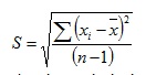
   where:
   xi = the analytical results in the final method reporting units for the eight replicate aliquots (i = 1 to 8)
    = the average of the eight replicate measurements

8. For option a) and b) above, for the assessment of historic within run replicate analysis data, calculate the standard deviation (S) of the replicate measurements as follows:

   

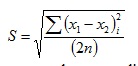
   where:
   x1, x2 = the two replicate results for each of the n replicate pairs (minimum n = 40)

9. Compute the MDL as follows:

   MDL = t(n-1, α = 0.01)S

   where: t(n-1,α 0.01) is the Student’s t value appropriate for a 99% confidence level given the degrees of freedom n-1.
   S = the standard deviation as determined above

   Tables of Student’s t Values at the 99% Confidence Level

   Number of Replicates	Degree of Freedom (n-1)	t (n-1)
   7	6	3.143
   8	7	2.998
   9	8	2.896
   10	9	2.821
   11	10	2.764
   16	15	2.602
   21	20	2.528
   26	25	2.485
   31	30	2.457
   ∞	∞	2.326

Recording

Record the calculated MDL to two significant figures (e.g. 0.032). The analytical method used must be specifically identified by number or title, and the MDL for each analyte expressed in the appropriate method reporting units. If the analytical method permits options which affect the MDL, these conditions must be specified with the MDL value. Report the mean analyte level with the MDL and indicate if the MDL procedure was iterated. If a laboratory standard, or a sample that contained a known amount of analyte, was used for this determination, also record the mean recovery.

Treatment of Outliers

Single Analyte Methods

If one of the results can be shown to be an 'outlier' by the Dixon test (described below), and the LMDL calculated for the remaining seven replicates (3.143 times S) is less than the RMDL, this latter estimate of the LMDL will be accepted.

Scans

Certain methods permit analysis of several analytes within a single 'scan'. The MDL for each analyte in the scan must be less than the corresponding RMDL. When the LMDLs tend to bracket the RMDLs, the overall method is not sensitive enough and, therefore, the LMDLs will not be considered acceptable.

However, if only a few of the LMDLs in a 'scan' exceed their respective RMDLs, there may be outliers within the set of eight replicates for these non-complying analytes. If this can be confirmed, as described above, for each of the non­complying analytes, then the LMDL based on seven replicates (3.143 times S) will be accepted for those few analytes.

To forestall the possibility that one replicate sample may be an outlier for all or most analytes in the scan, and that the calculated LMDLs will therefore be greater than the RMDL for several analytes, the analyst may choose the following option:

• perform 11 replicates (rather than eight);
• for each analyte, note which replicate gives the highest and the lowest results;
• reject the sample replicate containing the greatest number of high results;
• reject the sample replicate containing the greatest number of low results;
• reject the sample with the greatest number of high and low results; and,
• calculate LMDLs for each analyte using the remaining eight replicate samples.

If this procedure fails to indicate an LMDL for each analyte which is below the respective RMDL, redefine the method (for example, larger sample aliquot, different range expansion, etc.), retrain staff, and repeat the entire procedure for estimating RMDL for all analytes in the scan. Discard all previous replicate data.

Outlier procedure: Dixon’s Test for sample size n = 8 to 10.

1. sort the replicate values from lowest to highest r₁, r₂, … r_(n−1), r_n;
2. determine the difference between the suspect value and its nearest neighbour
   r₁ − r₂ (or r_n − r_(n−1),);
3. determine the difference between the suspect value and the next to last value at the opposite end of the sorted list of values r₁ − r_(n−1), (or r − r₂);
4. calculate the ratio of ii) divided by iii); and,
5. if the ratio is greater than 0.55, the value r₁ (or r_n) is considered to be an outlier
   (< 5% risk of error).

Natrella, M.G. "Experimental Statistics", NBS Handbook 91 (1966), USGPO, Washington, D.C.

Appendix 7: Ambient Monitoring Running Average Exceedances

This appendix has been prepared to clarify the requirements of reporting exceedances to the ministry using running averages, which is applicable for ambient monitoring data only. This guidance outlines the ministry’s minimum expectations with respect to reporting. It does not reference the total number of potential offences that may have occurred during an averaging period.

Section 3.1 of the Operations Manual stipulates that the requirements for reporting exceedances to the ministry are based on running averages, which are explained through different examples, as shown below. The examples are organised by averaging time, which in turn depend on the contaminant’s standard, guideline limit, or AAQC, and on whether O. Reg. 419/05 Schedule 2 or Schedule 3 applies.

Hourly Running Average

Hourly running averages may be computed from 1-minute or 5-minute data. Examples 1-3 illustrate 5-minute SO₂ average concentrations and resultant hourly running averages.

Example 1: SO₂ 1 Hr Running Avg.
1-hr Standard = 250 ppb

Date	Hour (EST)	5-min Avg. (ppb)	SO2 1-hr Runnning Avg. (ppb)
14-April	23:50	121	74
14-April	23:55	1392	75
15-April	00:00	1692	80
15-April	00:05	1922	87
15-April	00:10	2292	99
15-April	00:15	2682	115
15-April	00:20	2932	134
15-April	00:25	3042	155
15-April	00:30	3122	177
15-April	00:35	3162	199
15-April	00:40	3192	224
15-April	00:45	3262	249
15-April1	00:501	3812	2711
15-April	00:55	304	2845
15-April	01:00	286	2945
15-April	01:05	257	3003
15-April	01:10	234	3003
15-April	01:15	229	2975
15-April	01:20	221	2915
15-April	01:25	213	2835
15-April	01:30	218	2755
15-April	01:35	197	2655
15-April	01:40	176	2545
15-April	01:45	163	2404
15-April	01:50	152	221
15-April	01:55	148	208
15-April	02:00	121	194
15-April	02:05	117	182
15-April	02:10	94	171
15-April	02:15	89	159
15-April	02:20	37	144
15-April	02:25	39	129
15-April	02:30	45	115
15-April	02:35	48	102
15-April	02:40	59	93
15-April	02:45	76	85
15-April	02:50	92	80

In Example 1, 11 consecutive hourly running averages exceed the 250 ppb standard within a single averaging period, but this only constitutes a single exceedance. The exceedance would be reported as follows: An exceedance of the SO₂ 1-hour standard occurred at 00:50 EST on April 15 when the 1-hour running average was 271 ppb. During the exceedance period, successive running averages ranged between 240 ppb and 300 ppb.

Example 2: SO₂ 1 Hr Running Avg.
1-hr Standard = 250 ppb

Date	Hour (EST)	5-min Avg. (ppb)	SO2 1-hr Runnning Avg. (ppb)
09-September	06:25	106	117
09-September	06:30	113	114
09-September	06:35	119	113
09-September	06:40	126	113
09-September	06:45	1342	114
09-September	06:50	1622	117
09-September	06:55	1782	121
09-September	07:00	2032	129
09-September	07:05	2242	138
09-September	07:10	2392	149
09-September	07:15	2472	162
09-September	07:20	3342	182
09-September	07:25	3842	205
09-September	07:30	3672	226
09-September	07:35	3412	245
09-September1	07:401	3072	2601
09-September	07:45	2832	2725
09-September	07:50	2662	2815
09-September	07:55	2862	2905
09-September	08:00	2092	2913
09-September	08:05	1932	2885
09-September	08:10	1872	2845
09-September	08:15	1612	2775
09-September	08:20	2022	2665
09-September	08:25	2572	2555
09-September	08:30	2982	2495
09-September	08:35	3162	2474
09-September1	08:401	3622	2521
09-September	08:45	237	2485
09-September	08:50	213	2435
09-September	08:55	124	2305
09-September	09:00	298	2375
09-September	09:05	278	2445
09-September	09:10	261	2515
09-September	09:15	235	2575
09-September	09:20	213	2583
09-September	09:25	198	2535
09-September	09:30	168	2425
09-September	09:35	124	2264

In Example 2, the first hourly SO₂ exceedance occurred at 07:40 on September 9. It reflects a running average from 06:45 to 07:40. Although this period includes parts of two “clock” hours, it is 60 minutes long and thus is only one exceedance. Also, once a particular 5-minute value contributes to calculating an exceedance, it cannot be used to calculate a second exceedance. Therefore, the next 1-hour SO₂ exceedance cannot begin until one hour after the previous exceedance was determined, which in this case is at 08:40. The exceedance would be reported as follows: An exceedance of the SO₂ 1-hour standard occurred at 07:40 on September 9 when the 1-hour running average was 260 ppb. During the exceedance period, successive running averages ranged from a minimum of 247 ppb to a maximum of 291 ppb. This was immediately followed by a second exceedance which began at 08:40 on September 9, at which time the 1-hour SO₂ running average was 252 ppb. During this period, the concentration ranged between a minimum of 226 ppb and a maximum of 258 ppb.

Example 3: SO₂ 1 Hr Running Avg.
1-hr Standard = 250 ppb

Date	Hour (EST)	5-min Avg. (ppb)	SO2 1-hr Runnning Avg. (ppb)
12-August	14:10	98	133
12-August	14:15	106	129
12-August	14:20	109	125
12-August	14:25	114	123
12-August	14:30	119	121
12-August	14:35	125	121
12-August	14:40	127	122
12-August	14:45	139	123
12-August	14:50	147	124
12-August	14:55	159	125
12-August	15:00	162	127
12-August	15:05	174	132
12-August	15:10	181	139
12-August	15:15	189	145
12-August	15:20	1912	152
12-August	15:25	2292	162
12-August	15:30	2462	172
12-August	15:35	2892	186
12-August	15:40	3022	201
12-August	15:45	2842	213
12-August	15:50	2562	222
12-August	15:55	2312	228
12-August	16:00	2842	238
12-August	16:05	2562	245
12-August	16:10	2312	249
12-August1	16:151	2362	2531
12-August	16:20	184	2525
12-August	16:25	178	2485
12-August	16:30	234	2475
12-August	16:35	273	2465
12-August	16:40	297	2454
12-August	16:45	324	2495
12-August	16:50	316	2545
12-August	16:55	303	2603
12-August	17:00	258	2585
12-August	17:05	216	2545
12-August	17:10	176	2505

Example 3 illustrates that one exceedance period may incorporate periods where the average may exceed the standard or guideline, while others do not. However, all of these high values fall within a one hour span and use part of the data that resulted in the exceedance at 16:15. In this case, the exceedance would be reported as follows: An exceedance of the SO₂ 1-hour running average occurred at 16:15 on August 12 with a concentration of 253 ppb. During the exceedance period, running averages ranged from a minimum of 245 ppb to a maximum of 260 ppb.

Half-Hour Running Average

When reporting exceedances using half-hour running averages, the same principle as described above applies. That is, none of the data used to calculate one exceedance should be used for computing additional exceedances. The following examples illustrate 30-minute running average concentrations for NO₂.

Example 4: NO₂ ½ Hr Running Average
Half-hour Standard = 250 ppb

Date	Hour (EST)	5-min Avg. (ppb)	NO2 ½ Hr Running Avg. (ppb)
18-May	06:45	125	121
18-May	06:50	169	135
18-May	06:55	194	152
18-May	07:00	169	163
18-May	07:05	1942	174
18-May	07:10	2142	182
18-May	07:15	2392	197
18-May	07:20	2692	213
18-May	07:25	2962	230
18-May1	07:301	3082	2531
18-May	07:35	286	2695
18-May	07:40	254	2753
18-May	07:45	235	2755
18-May	07:50	221	2675
18-May	07:55	199	2514
18-May	08:00	171	228
18-May	08:05	149	205
18-May	08:10	126	184
18-May	08:15	105	162
18-May	08:20	84	139
18-May	08:25	77	119
18-May	08:30	61	100
18-May	08:35	57	85
18-May	08:40	55	73
18-May	08:45	49	64
18-May	08:50	56	59
18-May	08:55	72	58
18-May	09:00	86	63

Example 4 illustrates six consecutive 30-minute running averages within a half-hour period which results in one half-hour NO₂ exceedance at 07:30 on May 18. This exceedance would be reported as follows: An exceedance of the NO₂ half-hour standard occurred at 07:30 EST on May 18 with 253 ppb. During the exceedance period, successive running averages ranged from a minimum of 251 ppb to a maximum of 275 ppb.

Example 5: NO₂ ½ Hr Running Average
Half-hour Standard = 250 ppb

Date	Hour (EST)	5-min Avg. (ppb)	NO2 ½ Hr Running Avg. (ppb)
17-January	07:10	196	177
17-January	07:15	2142	190
17-January	07:20	2632	207
17-January	07:25	2712	224
17-January	07:30	2782	224
17-January	07:35	2642	248
17-January1	07:401	2372	2551
17-January	07:45	2262	2573
17-January	07:50	2352	2525
17-January	07:55	2472	2485
17-January	08:00	2612	2455
17-January	08:05	2482	2424
17-January1	08:101	3062	2541
17-January	08:15	2812	2633
17-January	08:20	1872	2555
17-January	08:25	2342	2534
17-January	08:30	2892	2585
17-January	08:35	2762	2625
17-January1	08:401	2542	2541
17-January	08:45	2412	2475
17-January	08:50	267	2605
17-January	08:55	2532	2633
17-January	09:00	2192	2524
17-January	09:05	3012	2565
17-January1	09:101	2862	2611
17-January	09:15	267	2663
17-January	09:20	242	2615
17-January	09:25	227	2575
17-January	10:25	224	2585
17-January	11:25	260	2514

Example 5, on the other hand, illustrates non-consecutive half-hour exceedances spread across half-hour clock-based periods. Example 5 illustrates a total of four exceedances, one at 07:40, the second at 08:10, the third at 08:40 and the fourth at 09:10, on January 17. The exceedances should be reported as follows: four NO₂ half-hour running average exceedances occurred on January 17 at 07:40, 08:10, 08:40, and at 09:10, at concentrations of 255, 254, 254 and 261 ppb, respectively. During the first exceedance event, NO₂ half-hour running averages ranged from a minimum of 242 ppb to a maximum of 257 ppb. During the second exceedance period, NO₂ half-hour running averages ranged from a minimum of 253 to a maximum of 263 ppb. The third exceedance event ranged from a minimum of 252 to a maximum of 263 ppb. The forth exceedance event ranged from a minimum of 251 to a maximum of 266 ppb.

Example 6: NO₂ ½ Hr Running Average
Half-hour Standard = 250 ppb

Date	Hour (EST)	5-min Avg. (ppb)	NO2 ½ Hr Running Avg. (ppb)
03-March	08:10	173	161
03-March	08:15	189	172
03-March	08:20	226	186
03-March	08:25	198	192
03-March	08:30	175	192
03-March	08:35	1972	193
03-March	08:40	2632	208
03-March	08:45	2572	219
03-March	08:50	2482	223
03-March	08:55	2892	238
03-March1	09:001	2962	2581
03-March	09:05	264	2703
03-March	09:10	238	2655
03-March	09:15	213	2585
03-March	09:20	206	2515
03-March	09:25	197	2364
03-March	09:30	176	216
03-March	09:35	203	206
03-March	09:40	2142	202
03-March	09:45	1932	198
03-March	09:50	2552	206
03-March	09:55	2962	223
03-March	10:00	2962	243
03-March1	10:051	2722	2541
03-March	10:10	241	2595
03-March	10:15	228	2653
03-March	10:20	202	2565
03-March	10:25	197	2395
03-March	10:30	176	2194

Example 6 illustrates non-consecutive half-hour exceedances resulting in two exceedances: one at 09:00 and the second at 10:05 on March 3. The exceedances should be reported as follows: There were two NO₂ half-hour running average exceedances that occurred on March 3 at 09:00 and 10:05 with concentrations of 258 and 254 ppb, respectively. The first exceedance episode ranged from a concentration of 236 ppb to a maximum of 270 ppb. The second exceedance event included 5-minute values that ranged from a minimum of 219 ppb to a maximum of 265 ppb.

Ten-Minute Running Average

The same reporting principle applies to exceedances of 10-minute standards such as total reduced sulphur (TRS) compounds. Examples 7 through 9 illustrate 10-minute running averages for TRS concentrations.

Example 7: TRS 10 Min Running Average
10-min Standard = 9 ppb

Date	Hour (EST)	5-min Avg. (ppb)	TRS 10-min Running Avg. (ppb)
06-June	07:20	0.0	0.0
06-June	07:25	0.0	0.0
06-June	07:30	0.0	0.0
06-June	07:35	0.0	0.0
06-June	07:40	0.0	0.0
06-June	07:45	3.2	1.6
06-June	07:50	13.02	8.1
06-June1	07:551	21.02	17.01,3
06-June	08:00	9.02	15.04
06-June1	08:051	32.02	20.51,3
06-June	08:10	8.02	20.04
06-June1	08:151	28.02	18.01,3
06-June	08:20	7.02	17.54
06-June1	08:251	26.02	16.51,3
06-June	08:30	5.02	15.54
06-June1	08:351	21.02	13.01,3
06-June	08:40	4.02	12.54
06-June1	08:451	15.02	9.51,3
06-June	08:50	2.0	8.54
06-June	08:55	7.0	4.5
06-June	09:00	3.0	5.0
06-June	09:05	14.0	8.5
06-June	09:10	2.0	8.0
06-June	09:15	4.0	3.0
06-June	09:20	0.0	2.0
06-June	09:25	0.0	0.0

Example 7 illustrates six 10-minute TRS exceedances spread across multiple clock periods: 07:55, 08:05, 08:15, 08:25, 08:35 and 08:45 on June 6. During the exceedance period, successive running averages ranged from a minimum of 8.5 ppb to a maximum of 20.5 ppb.

Example 8: TRS 10 Min Running Average
10-min Standard = 9 ppb

Date	Hour (EST)	5-min Avg. (ppb)	TRS 10-min Running Avg. (ppb)
04-October	08:05	0.0	0.0
04-October	08:10	0.0	0.0
04-October	08:15	0.0	0.0
04-October	08:20	0.0	0.0
04-October	08:25	0.0	0.0
04-October	08:30	0.0	0.0
04-October	08:35	0.0	0.0
04-October	08:40	0.0	0.0
04-October	08:45	5.1	2.6
04-October	08:50	9.42	7.3
04-October1	08:551	15.12	12.31,3
04-October	09:00	7.7	11.44
04-October	09:05	10.0	8.9
04-October	09:10	0.6	5.3
04-October	09:15	0.0	0.3
04-October	09:20	0.0	0.0
04-October	09:25	0.0	0.0
04-October	09:30	0.0	0.0
04-October	09:35	0.0	0.0
04-October	09:40	0.0	0.0
04-October	09:45	0.0	0.0
04-October	09:50	0.0	0.0
04-October	09:55	0.0	0.0
04-October	10:00	0.0	0.0
04-October	10:05	0.0	0.0
04-October	10:10	0.0	0.0

Example 8 shows a 10-minute TRS exceedance which crosses between two clock-based periods. In this example only one 10-minute TRS exceedance at 08:55 on October 4 should be reported. The 10-minute TRS running average at 09:00 is not a second exceedance, since the 5-minute data used for the computation was part of the previous 10-minute TRS exceedance. The exceedances should be reported as follows: There was one TRS 10-minute running average exceedance that occurred on October 4 at 08:55 with 12.3 ppb. The exceedance period included concentrations ranging from a minimum of 11.4 ppb to a maximum of 12.3 ppb.

Example 9: TRS 10 Min Running Average
10-min Standard = 9 ppb

Date	Hour (EST)	5-min Avg. (ppb)	TRS 10-min Running Avg. (ppb)
05-December	09:30	0.0	0.0
05-December	09:35	0.0	0.0
05-December	09:40	3.9	1.9
05-December	09:45	7.92	5.9
05-December1	09:501	14.32	11.11,3
05-December	09:55	7.2	10.84
05-December	10:00	9.62	8.4
05-December1	10:051	9.42	9.51,3
05-December	10:10	8.4	8.94
05-December	10:15	2.4	5.4
05-December	10:20	15.22	8.8
05-December1	10:251	7.82	11.251,3
05-December	10:30	13.2	10.54
05-December	10:35	5.4	9.3
05-December	10:40	2.3	3.9
05-December	10:45	1.6	2.0
05-December	10:50	4.3	3.0
05-December	10:55	5.8	5.1
05-December	11:00	7.6	6.7
05-December	11:05	8.9	8.3
05-December	11:10	4.2	6.6
05-December	11:15	0.0	2.1
05-December	11:20	0.0	0.0
05-December	11:25	0.0	0.0
05-December	11:30	0.0	0.0
05-December	11:35	0.0	0.0

Example 9 illustrates blocks of time that include non-consecutive exceedances, calculated from running averages, which occur across and within a 10-minute clock based period. Example 9 illustrates three 10-minute TRS exceedances, which are at 09:50, 10:05 and 10:25 on December 15. The exceedances should be reported as follows: There are three TRS 10-minute running average exceedances which occurred on December 15; at 09:50, 10:05 and 10:25, with concentrations of 11.1, 9.5 and 11.5 ppb, respectively. During the exceedance period, successive running averages ranged from a minimum of 8.9 ppb to a maximum of 11.5 ppb.

24-Hour Running Average

Daily running averages may be calculated from 1-hour averages. Examples 10 through 12 illustrate 24-hour PM₁₀ running averages within and across 24-hour clock-based periods.

Example 10: PM₁₀ 24 Hr Running Average
Daily AAQC = 50 µg/m³

Date	Hour (EST)	1-Hour Avg. (µg/m3)	PM10 24-Hr Running Avg. (µg/m3)
06-May1	03:001	1482	561
06-May	04:00	123	605
06-May	05:00	107	635
06-May	06:00	95	655
06-May	07:00	84	675
06-May	08:00	68	685
06-May	09:00	52	693
06-May	10:00	43	693
06-May	11:00	39	693
06-May	12:00	32	693
06-May	13:00	26	685
06-May	14:00	55	693
06-May	15:00	66	693
06-May	16:00	47	675
06-May	17:00	36	655
06-May	18:00	27	615
06-May	19:00	21	595
06-May	20:00	34	575
06-May	21:00	28	555
06-May	22:00	19	545
06-May	23:00	17	535
07-May	00:00	14	515
07-May	01:00	15	515
07-May	02:00	12	504
07-May	03:00	18	45
07-May	04:00	23	41
07-May	05:00	27	37
07-May	06:00	24	34
07-May	07:00	21	32
07-May	08:00	24	30
07-May	09:00	19	29

Example 10 illustrates one 24-hour PM₁₀ non-conformance on May 6 at 03:00. In this case, the next non-conformance cannot occur until at least 24 hours after the first non-conformance, on May 7 at 03:00. The exceedances should be reported as follows: There was one 24-hour PM₁₀ running average non-conformance that occurred on May 6 at 03:00 with a concentration of 56 µg/m³. During the non-conformance period, daily running averages ranged from a minimum of 50 µg/m³ to a maximum of 69 µg/m³.

Example 11: PM₁₀ 24 Hr Running Average
Daily AAQC = 50 µg/m³

Date	Hour (EST)	1-Hour Avg. (µg/m3)	PM10 24-Hr Running Avg. (µg/m3)
16-July	21:00	462	47
16-July	22:00	572	48
16-July	23:00	522	49
17-July1	00:001	592	511
17-July	01:00	56	525
17-July	02:00	48	535
17-July	03:00	36	535
17-July	04:00	26	535
17-July	05:00	22	525
17-July	06:00	56	535
17-July	07:00	63	545
17-July	08:00	58	555
17-July	09:00	58	565
17-July	10:00	59	575
17-July	11:00	60	575
17-July	12:00	63	583
17-July	13:00	63	583
17-July	14:00	56	583
17-July	15:00	52	583
17-July	16:00	57	583
17-July	17:00	44	555
17-July	18:00	37	535
17-July	19:00	32	525
17-July	20:00	24	495
17-July	21:00	21	485
17-July	22:00	17	475
17-July	23:00	14	454
18-July	00:00	17	43
18-July	01:00	19	42
18-July	02:00	21	41
18-July	03:00	27	40

Example 11 illustrates a 24-hour period where 20 of the hours had values above the PM₁₀ benchmark. In this example, there is one daily PM₁₀ non-conformance of the AAQC which occurred at midnight (00:00), with a concentration of 51 µg/m³. During the non-conformance period, daily running averages ranged from a minimum of 45 µg/m³ to a maximum of 58 µg/m³.

Example 12: PM₁₀ 24 Hr Running Average
Daily AAQC = 50 µg/m³

Date	Hour (EST)	1-Hour Avg. (µg/m3)	PM10 24-Hr Running Avg. (µg/m3)
10-August	23:00	1292	39
11-August	00:00	1182	43
11-August	01:00	962	46
11-August	02:00	792	49
11-August1	03:001	1262	541
11-August	04:00	83	565
11-August	05:00	81	595
11-August	06:00	45	605
11-August	07:00	21	605
11-August	08:00	25	605
11-August	09:00	27	605
11-August	10:00	36	615
11-August	11:00	49	625
11-August	12:00	31	633
11-August	13:00	23	625
11-August	14:00	27	625
11-August	15:00	16	625
11-August	16:00	11	615
11-August	17:00	19	605
11-August	18:00	17	585
11-August	19:00	13	555
11-August	20:00	9	515
11-August	21:00	7	495
11-August	22:00	16	465
11-August	23:00	10	415
12-August	00:00	8	365
12-August	01:00	9	335
12-August	02:00	14	304
12-August	03:00	21	26
12-August	04:00	29	24
12-August	05:00	33	22
12-August	06:00	28	21

Example 12, on the other hand, illustrates a 24-hour period that contains non-consecutive running averages which are higher than the benchmark and span two calendar days. However, only one 24-hour PM₁₀ non-conformance should be reported in Example 12, which occurred on August 11 at 03:00, with a concentration of 54 µg/m³. During the non-conformance period, daily running averages ranged from a minimum of 30 µg/m³ to a maximum of 63 µg/m³.

Glossary of Terms

Audit

A check by ministry staff of the performance of an air quality monitoring system operated by the emitter or their site operator. The field component of the audit consists of assessing compliance/conformance of the sites with established criteria, and in conducting instrument performance checks with certified calibration devices to ensure that the instruments are operating within acceptable tolerances. The other component consists of reviewing documents and procedures to ensure that proper information management practices/procedures have been implemented by the emitter or its site operator, and are followed.

Calibration Check

A test of the accuracy of an instrument using a certified calibration device traceable to a primary standard. If the difference in accuracy between the instrument and the calibration device is greater than ±5%, a calibration of the instrument should be performed.

Calibration

An instrument adjustment with a certified calibration device traceable to a primary standard following an audit or a calibration check when the accuracy of the instrument deviates by more than 5% from the required set point. Instrument calibrations are performed by site operators and not by the inspectors.

Certification of calibrators

A test of the accuracy of a calibration device traceable to a primary standard. At least once per year, formal certification of calibration devices by a certification authority is required.

Continuous monitoring

Monitoring performed with fully automated instrumentation that collects data on a very short time scale (e.g., every second or minute) such as an ozone or sulphur dioxide analyzer thereby providing realtime data.

Cycling time

The time required to complete the active measurement cycle (sample collection, analysis and measurement) and to produce an output.

Emitter

The person in occupation or having the charge, management or control of a facility that emits air contaminants into the natural environment.

External performance check

QA/QC procedure carried out external to an instrument with a certified calibration unit (e.g., calibrator, gas cylinder, etc., referenced to a primary standard). It is synonymous to a calibration check.

Fall time to 95%

The time interval between initial response (the first observable change in analyser output) and a level of signal output, which is 95% of the steady state output after a step decrease in input concentration.

Internal performance check

QA/QC procedure carried out ‘within’ the analyzer and, as such, consists in all instruments checks not done with a calibrator.

Linearity

The maximum deviation between the actual analyser output reading and the predicted analyser output from a least square fit to the actual readings.

Minimum Detection Limit

The lowest concentration that can be detected by the analyser with confidence. It is defined as twice the noise level of the analyser.

Noise

Spontaneous short duration deviations in the analyser output, about the mean output, which are not caused by input concentration changes.

Non-continuous sampling

Sampling conducted with discrete samplers that collect a sample, typically over a 24-hour period such as a Hi-Vol sampler. Samples are collected on a set schedule, such as once every 6^th day.

Operating humidity range

The maximum level of moisture content of the ambient air in the environment surrounding the analyser, in which the analyser will meet all performance specifications.

Operating Ranges

The ranges corresponding to the full-scale output of the analyser.

Operating Voltages

The minimum and maximum line voltages in which the analyser will meet all performance specifications.

Operating temperature range

The minimum and maximum ambient temperature, of the environment surrounding the analyser, in which the analyser will meet all performance specifications.

Precision

The degree of variation about the mean of repeated measurements of the same pollutant concentration by the analyser, expressed as standard deviation about the mean.

Primary standard

The reference standards used by the United States National Institute of Standards and Technology (NIST) against which other standards (secondary) are compared with for accuracy. The certification of calibration devices used must be traceable to a primary standard through secondary standards.

Probe

Sampling inlet; The point of entry of an air sample into an air quality monitoring system. A probe’s siting must meet criteria to ensure that a representative and unbiased sample is collected.

Proponent

A person or organization that has established or is undertaking air monitoring other than the MOECC or an emitter, or contractor employed by an emitter, as defined herein.

Rise time to 95%

The time interval between initial response (the first observable change in analyser output) and a level of signal output, which is 95% of the steady state output after a step increase in input concentration.

Running Average

A running average is a calculation to analyse data points by creating a series of different subsets of the full data set. It is also called a moving mean or a rolling mean.

Span Drift

The percent change in analyser output response to a constant upscale pollutant concentration over a period of unadjusted continuous operation.

Station operator

The person that performs the regular operation and maintenance of the station. This can be the emitter or a third party retained by the emitter.

Verification of Calibrators

A check of the gas calibration devices used by site operators in the field by ministry audit staff with their calibrators. This is to be done between the annual formal certifications and does not constitute a certification.

Zero Drift

The change in analyser output response to a constant zero air input concentration over a period of unadjusted continuous operation.

Acronyms

AAQC

Ambient Air Quality Criteria as defined and listed in O. Reg. 419/05

AAQD

Analysis and Air Quality Division of Environment Canada

ASTM

American Society for Testing and Materials

BAM

Beta Attenuation Monitor, more commonly known as a beta gauge monitor used to measure (in real-time) concentrations of particulate matter, mostly in the PM₁₀ and PM_2.5 size fractions

BIOS

Acronym for basic input/output system, the built-in software that determines what a computer can do without accessing programs from a disk.

CALA

Canadian Association for Laboratory Accreditation

CAMM

Combined Assessment of Modelling and Monitoring; a study conducted under O. Reg. 419/05, Section 11(1), Paragraph 3, with the purpose of refining emission rates for modelling

cm³/min

Cubic centimetres per minute

cfm

Cubic feet per minute

CFR

Code of Federal Regulations (U.S.)

CST

Central Standard Time

CSV

Comma Separated Values. A data format with values separated by a comma

DAS

Data Acquisition System. The hardware/software of a system used to collect data electronically

Delta Cal

Trade name for a device used to calibrate flow, temperature and ambient pressure

ΔP

Pressure differential

DVM

Digital voltmeter

EA

Environmental Assessment

ECA

Environmental Compliance Approval

ECCC

Environment and Climate Change Canada (formerly Environment Canada)

EMRB

The Environmental Monitoring and Reporting Branch of the ministry

ESDM

Emission Summary and Dispersion Modelling Report. This is one of the key documents required in the application package for an Air Certificate of Approval from the ministry

EST

Eastern Standard Time

FEP

Fluorinated ethylene propylene

GC-MS

Gas chromatography and mass spectrometry

GIS

Geographic Information System

H₂S

Hydrogen sulphide

I.D.

Inside diameter

in. of Hg

Inches of mercury (unit of barometric pressure)

km/hr

Kilometres per hour

L/min

Liters per minute

LaSB

Laboratory Services Branch of the ministry

LCD

Liquid crystal display

m³

Cubic metre

MDL

Method Detection Limit (analytical lab methods). In this document it is defined as the smallest measurable amount, where the risk of a false positive is 1%, or conversely the confidence level is 99%.

mL/min

Milliliters per minute

MOECC

Ministry of the Environment and Climate Change (Ontario)

NIST

United States National Institute of Standards and Technology (NIST) which is the source of the primary reference standards for the monitoring/sampling methods listed in this document

NO

Nitric oxide

NO₂

Nitrogen dioxide

NO_x

Oxides of nitrogen, principally nitric oxide (NO) and nitrogen dioxide (NO₂)

O.D.

Outside diameter

ng/m³

nanograms per cubic metre

PAH

Polycyclic aromatic hydrocarbons

PCDD

Polychlorinated dibenzo-p-dioxins, commonly known as dioxins

PCDF

Polychlorinated dibenzofurans, commonly known as furans

PDF

Portable document format

PM₁₀

Particulate matter with an aerodynamic diameter less than about 10 microns; also known as inhalable particulate matter

PM_2.5

Particulate matter with an aerodynamic diameter less than about 2.5 microns; also known as fine particulate matter or respirable particulate matter

POI

Point of Impingement as defined in O. Reg. 419/05

ppbv

Concentration of a gaseous contaminant expressed in parts per billion by volume of air sampled

pg/m³

Concentration of an air contaminant expressed in picograms (10⁻¹² gram) per cubic metre of air sampled

PUF

Polyurethane Foam cartridge used for the determination of polycyclic aromatic hydrocarbons (PAHs), dioxins (PCDDs) and furans (PCDFs) in air

QA/QC

Quality Assurance and Quality Control programs to ensure the collection and reporting of data of acceptable quality

RFP

Request for proposal

RTD

Resistance temperature detector

SCC

Standards Council of Canada which accredits analytical laboratories in Canada

SO₂

Sulphur dioxide gas

SOP

Standard Operating Procedure for monitoring/sampling of air contaminants

SHARP

Synchronised Hybrid Ambient Real-time Particulate

SP

Suspended Particulate matter is all airborne, finely divided solid or liquid material. Some particles, such as dust, dirt, soot, or smoke, are large or dark enough to be seen with the naked eye. Others are so small that individual particles can only be detected using microscopy techniques. See Particulate Matter (PM) Basics

STEM

Station Temperature (for Air Quality Monitoring stations)

TEOM

Tapered Oscillating Microbalance. A particulate monitor for determining (in real-time) concentrations of particulate matter, mostly in the PM₁₀ and PM_2.5 size fractions

TEQ

Toxicity Equivalent values are obtained by determining the relative toxicity of a doxin or furan congener to that of 2,3,7,8-TCDD (tetrachlorodibenzo-p-dioxin) and using these factors for each of the members of a mixture to assign a toxicity to the whole.

TFE

Tetrafluoroethylene

TriCal

Trade name for a device used to calibrate flow, temperature and ambient pressure

TRS

Total Reduced Sulphur compounds consisting mostly of hydrogen sulphide (H₂S) and mercaptans

TRST

Total Reduced Sulphur Temperature (temperature of high temperature TRS converter)

US EPA

United States Environmental Protection Agency

URT

Upper Risk Thresholds for air contaminants as listed in schedule 6 of O. Reg. 419/05

UV

Ultraviolet light

µg/m³

Microgram (10⁻⁶ gram) per cubic metre of air sampled

µm

Micron (or micrometre) which is 10⁻⁶ of a metre

VOC

Volatile Organic Compounds some of which play an important role in the formation of ozone and smog aerosols

VWSA

Vertical Wind Speed Average

WINS

Well Impactor Ninety Six, an impactor designed to provide a particle cut-point of 2.5 microns

WMO

World Meteorological Organization

References

¹ National Air Pollution Surveillance Network Quality Assurance and Quality Control Guidelines, Environment Canada, Environment Protection Service, Environmental Technology Advancement Directorate, Pollution Measurement Division, Environmental Technology Centre, Ottawa, Ontario. Report No. AAQD 2004-1 (Originally published as Report No. PMD 95-8, December 1995).

² ISO/IEC17025:2005 - General Requirements for the Competence of Testing and Calibration Laboratories. Available at ANSI webstore.

³ U.S. Code of Federal Regulations, Title 40, Volume 5, Part 58, Appendix D (Network Design Criteria for Ambient Air Quality Monitoring) and Appendix E (Probe and Monitoring Path Siting Criteria),EPA 1999. Revised July 1, 1999.

⁴ Meteorological Monitoring Guidance for regulatory Modeling Applications. EPA 2000. EPA-454/R-99-005, Section 3 (Siting and Exposure), February 2000.

⁵ Guide to Meteorological Instruments and Methods of Observation. WMO 2008. World Meteorological Organization-No. 8, 7^th edition, Geneva Switzerland.