Measuring field slopes for nutrient management and conservation planning

Introduction

The topography of a field greatly determines how susceptible the soil is to erosion by water. In general, the steeper and longer the slopes are in a field, the greater the soil erosion potential. Eroded soil carries away organic-rich topsoil and its valuable crop nutrients.

To estimate a field’s long-term average soil erosion rate, soil conservation planners and agronomists often use the Universal Soil Loss Equation (USLE), or an updated version of this equation called the Revised Universal Soil Loss Equation (RUSLE2).

The USLE is used as the default method in various nutrient management and soil and water conservation planning tools available in the Ministry of Agriculture, Food and Rural Affairs’ (OMAFRA) AgriSuite. For example, PLATO (the Phosphorus Loss Assessment Tool for Ontario), included in AgriSuite, gives users an estimate of the relative soil loss and associated phosphorus loss potential for a field managed under different cropping and management practices.

Both the USLE and RUSLE2 require information on a field’s slope as input to complete the calculations. It can be difficult to get an accurate slope value given that there are many hillslope measurement locations in a single field.

The following information will guide users in determining suitable slope length and gradient values to describe a field.

Definitions

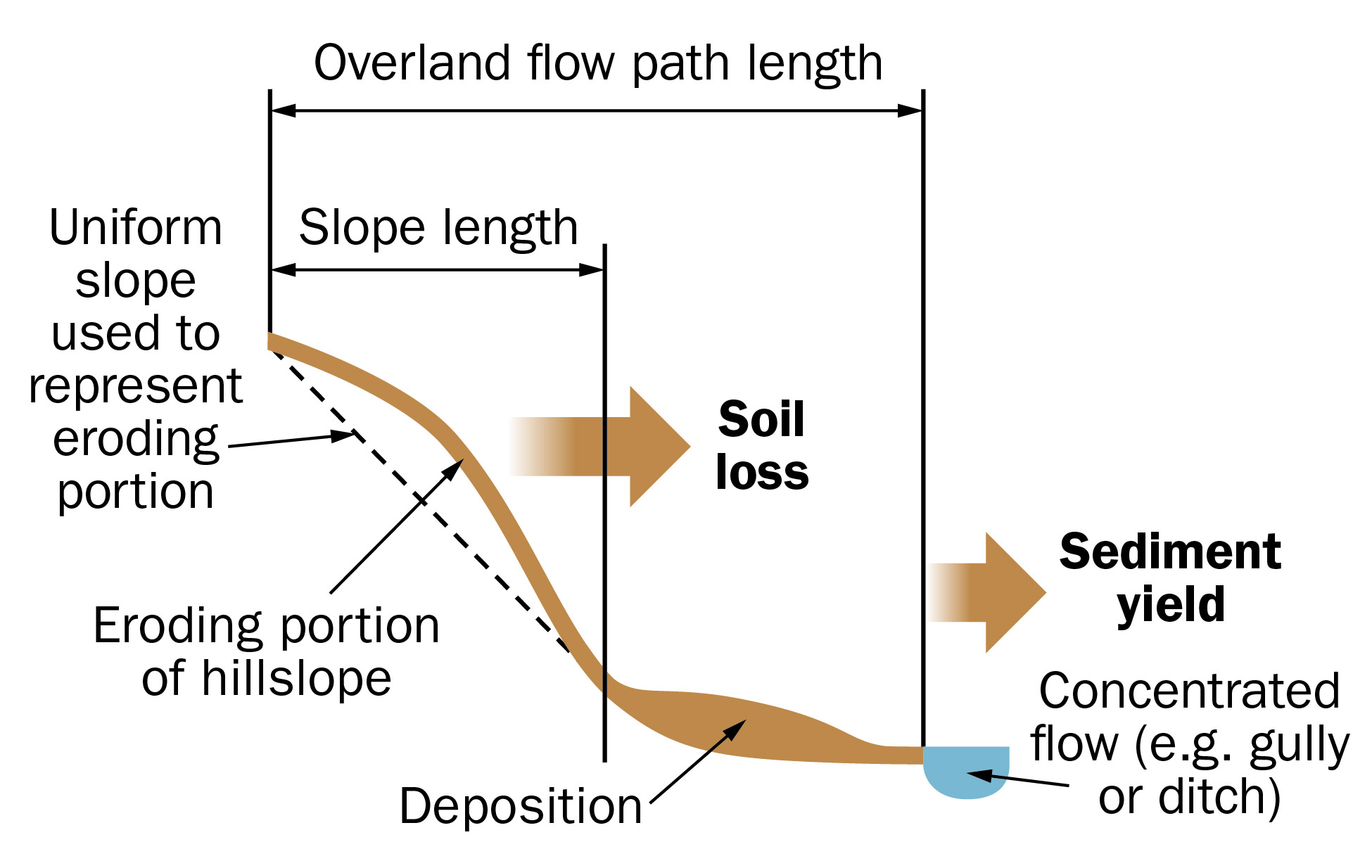
To begin, it is important to understand how erosion estimation equations define a field slope for the purpose of making estimates of soil erosion. For all definitions, runoff along a hillslope is assumed to be perpendicular to the hillslope contours. The USLE defines a slope length as the distance from the highest point of origin of overland flow to the point where deposition begins. This traditional definition of field slope length can be used as slope length input to either the USLE equation or the RUSLE2 equation.

RUSLE2 can also accommodate a more complex description of field slope called the overland flow path length. The overland flow path length is the distance runoff water travels as it moves across a field’s soil surface from its highest point of origin to the point where it becomes concentrated flow, such as in a grassed waterway or open ditch.

Figure 1 shows the difference between the USLE slope length definition and the overland flow path slope length definition that is represented in RUSLE2. The USLE definition of slope length stops where deposition begins. As a rule, deposition along a slope length in a field is assumed to begin at the point where slope steepness is half of the average steepness of the field slope above this point.

Normally, slope is measured as the elevation drop along an average straight-line distance (dotted line on each drawing in Figure 2). Figure 2 shows that overland flow paths can have a variety of shapes and the slope gradients along that distance can vary.

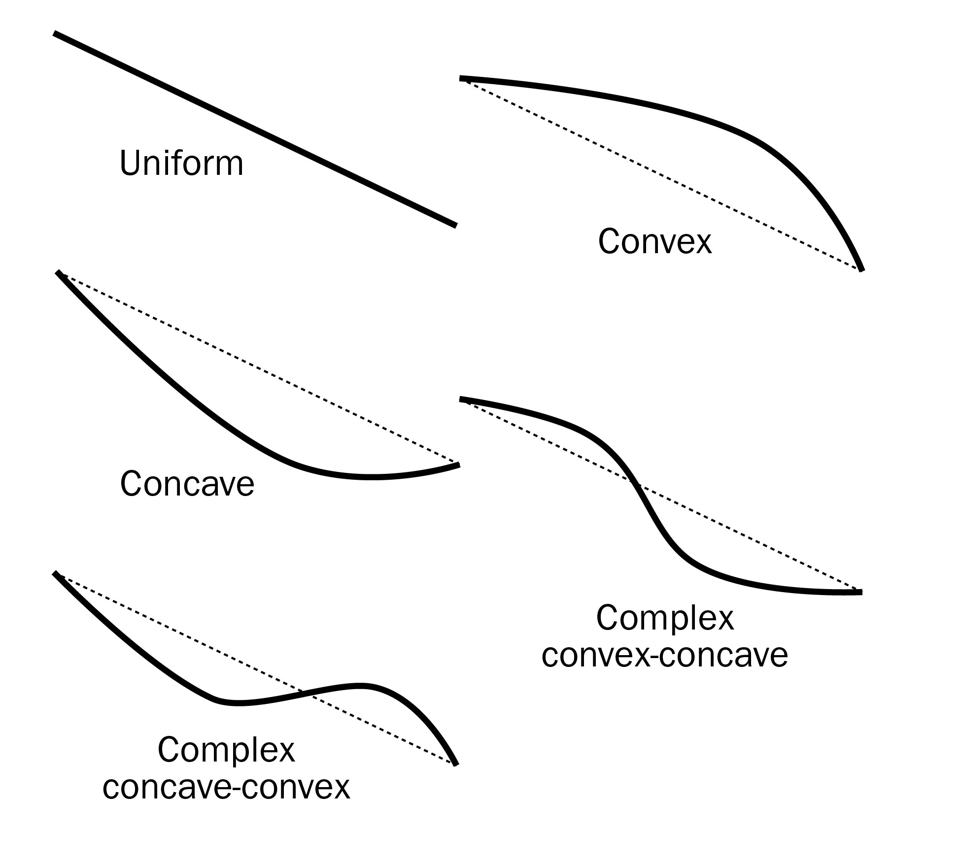
RUSLE2 can operate using the USLE definition of slope length and allows users to input various slope shapes such as shown in Figure 2, which may be more representative of the actual shape of the entire overland flow path. In this way, RUSLE2 can estimate the rate of soil erosion or deposition occurring at any point along the length of the overland flow path. With this capability, RUSLE2 can estimate the net amount of sediment that is ultimately delivered to the bottom of an overland flow path and that enters the concentrated flow area, such as a gully, watercourse or sediment pond (Figure 3).

For Ontario nutrient management planners, it is important to be aware of the difference between the USLE/RUSLE2 definitions of slope and flow path and the province’s nutrient management regulation’s definition of similar terms. O. Reg. 267/03 defines a “flow path” in Section 1.1 as follows: “'Flow path,' in relation to a facility, site, outdoor confinement area, temporary storage area or vegetated filter strip system, means a surface channel or depression that conducts liquids away from the facility, site, area or system.”

This regulatory definition is focused more on flow paths associated with sites where prescribed materials such as manure are being produced or stored. The USLE/RUSLE2 definition of flow path is much broader than the nutrient management regulatory definition in that it includes any pathway in a cropped field that rainfall or snowmelt runoff follows or collects in while carrying eroded soil.

The nutrient management regulation also refers to a maximum sustained slope within 150 m (492 ft) of a watercourse and defines this maximum sustained slope as “the change in elevation from the top to the bottom of a slope divided by the length of the slope expressed as a percentage, where the slope has a minimum length of 10 m (33 ft) and where the slope is towards surface water.”

This definition describes the maximum sustained slope as a simple straight line or “uniform” slope as opposed to a more complex slope shape (Figure 2). Unlike the standard USLE uniform slope that would end at the point where sedimentation begins (Figure 1), the “maximum sustained slope” is averaged over the entire length of the flow path to the point where it terminates at surface water. Section 1 of the nutrient management regulation further defines surface water and, as part of that definition, excludes features such as grassed waterways, shallow temporary channels, roadside ditches, rock chutes and temporarily ponded areas that are normally farmed, as being surface water. A USLE uniform slope or RUSLE2 complex slope, on the other hand, would terminate at the point where a hillside slope enters features such as a waterway or man-made temporary scrape ditch in a field.

Methods to determine slope

There are a variety of tools and approaches that can be used to measure field slopes.

The simplest approach for estimating slope gradient is to obtain a copy of the soils report for the county where the field is located. OMAFRA’s online geographic information portal, AgMaps, provides this same information if a hard-copy soils map is not available.

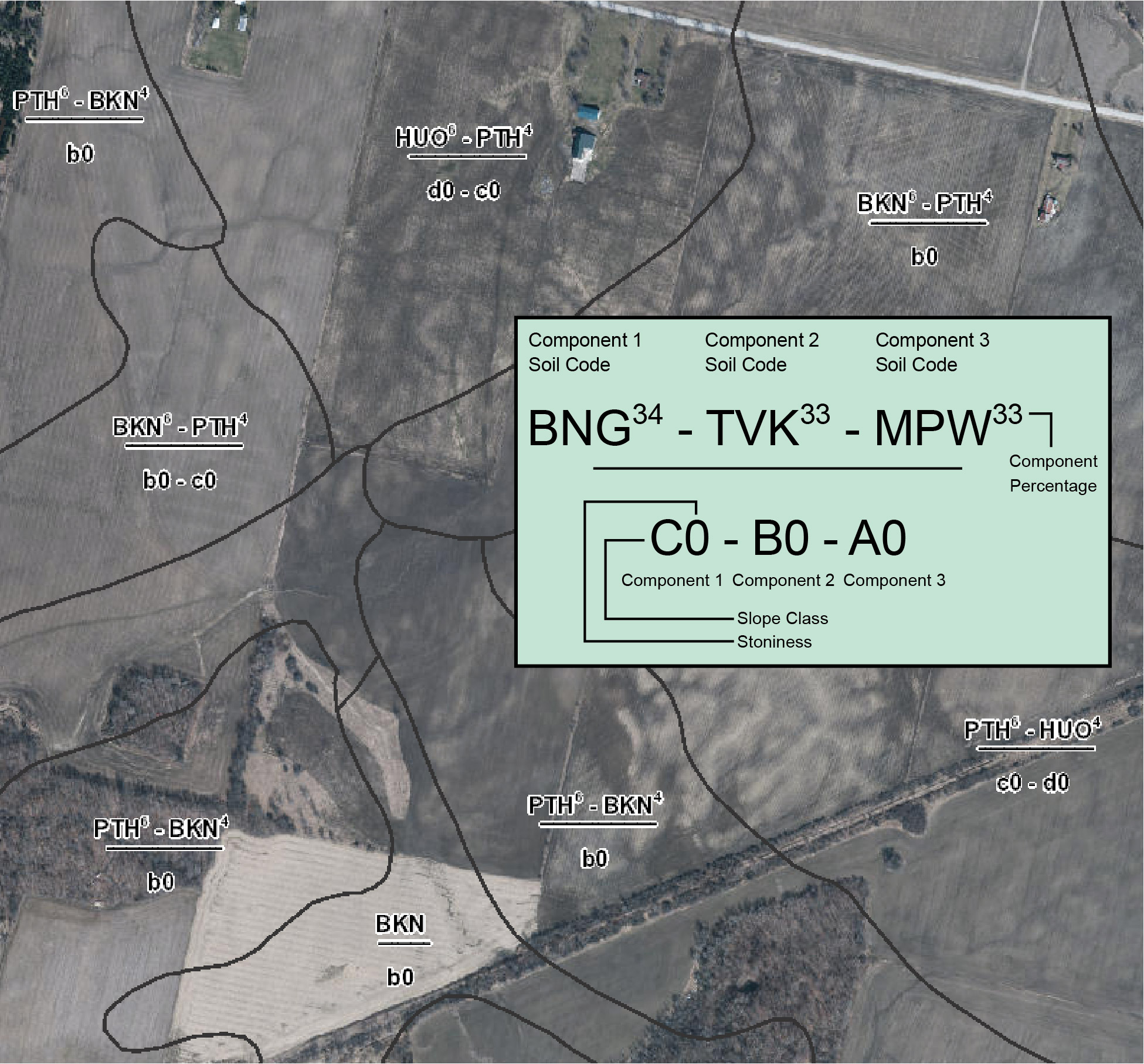
Figure 4 gives an example of an area in Middlesex County showing the soil code information as displayed in AgMaps. This “soil code” includes a code for the slope class in the code’s denominator. The inset in Figure 4 shows where within the soil code the slope class is listed. Note that up to three different soil types can be identified in a soil code. For the Middlesex example, only one or two soil types were listed in the soil code for each soil polygon. Slope classes in most Ontario soil reports are defined in Table 1.

Table 1. Slope classes in Ontario soil reports

Class	Percent slope %	Description
A	0.0–0.5	Level
B, b	0.5–2	Nearly level
C, c	2–5	Very gently sloping
D, d	5–9	Gently sloping
E, e	9–15	Moderately sloping
F, f	15–30	Strongly sloping
G, g	30–45	Very strongly sloping

Slope length is difficult to obtain solely from a soil map. Uppercase letters used for the slope class presented in Table 1 suggest the soil polygon has slopes that are more than 50 m (160 ft) in length. Lowercase letters indicate the slope lengths are less than 50 m (160 ft).

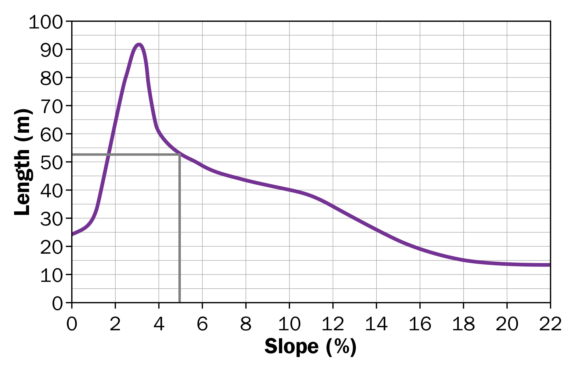
Soil conservation planning practitioners in the United States, who have measured slope length and gradient in the field for years, have developed a way to approximate the USLE-related slope length from known slope gradients. Figure 5 shows this relationship of maximum slope length for a given slope gradient. For example, if a 5% slope gradient is measured, the maximum slope length that is typically expected before the flow becomes concentrated is 53 m (175 ft). This is the default approach used in OMAFRA’s Agrisuite.

Another useful way to calculate the length and gradient of field slopes is to use information from prepared topographic contour maps. Contour maps, or at least the datapoints needed to prepare detailed contour mapping, can be obtained from a variety of sources, including:

• tile drainage installation mapping
• Digital Elevation Model (DEM) data originating from a variety of elevation data collection sources, including:
  • precision farming tools that collect Real Time Kinematic (RTK) field positioning data that are also accurate in the vertical or “Z” direction
  • published digital elevation data such as is available though the Ontario GeoHub or
  • direct field measurement made using Light Detection and Ranging (LiDAR) field equipment or traditional laser or field surveying equipment

Figure 6 is an example of a detailed contour map of an area of a field, prepared using LiDAR data. The thin red lines are the contour lines for the field. The assumed elevation of the contour is given by the red number located just above each contour line. The closer contour lines are to each other, the steeper the field’s slopes. For this example, the contours are at 0.3 m (1 ft) intervals.

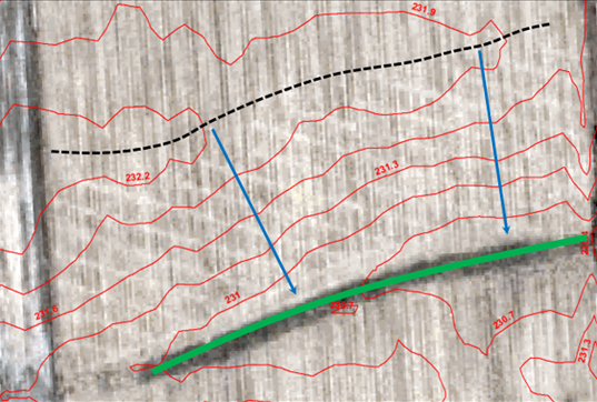
The thick green line in Figure 6 marks the concentrated flow pathway — a grassed waterway in this case — that the hillside slopes drain toward. The high point, or sub-watershed boundary, is shown by the dashed black line. This marks the high or starting point for the hillside slope. The blue arrows on the map that run approximately perpendicular to the contour lines between the highpoint and the grassed waterway represent the hillside’s overland flow path. The length and gradient of these flow pathways can be used as length and slope input into USLE or RUSLE2. In this example, the blue lines are approximately 90 m (295 ft) long, and the elevation difference between the top and bottom of the hillslope is approximately 232.2 – 230.7 = 1.5 m (5 ft). The slope is therefore 1.5/90 = 1.7%.

Direct field measurements can also be taken to determine slope length and gradient when no mapping is available. Tools for directly measuring slope length include a distance measuring wheel, a steel or fibreglass tape, pacing (provided you have calibrated your steps to a known distance), a hand-held GPS device, or a laser range finder.

Measuring slope steepness can be done using a hand-held Abney level or clinometer. They are available for purchase online. Abney levels and clinometers may have 2 scales: percent and degrees. Slope, for erosion estimation purposes, is measured using the percent scale. Several free apps are also available for mobile phones that can be used as a handheld device to measure slope. However, verify these measurements as it can be difficult to hold the phone in a way that both measures slope and provides an accurate reading. For any of these handheld slope measurement tools, be sure to establish the height of your eye level and use this height as a target on the bottom or top end of the slope being measured.

Where to measure field slope

Given the range of topography in most fields, it can be difficult to decide which slope to measure or from where in the field to measure the slopes.

O. Reg. 267/03 requires the maximum sustained slope that is within 150 m (492 ft) of surface water be the slope(s) measured.

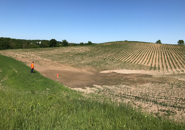
For USLE/RUSLE2-related soil erosion estimation, the United States Department of Agriculture’s Natural Resources Conservation Service (USDA-NRCS) recommends using the hillside flow path profile that represents the topography of one-third to one-quarter of the most erodible part of the field. Figure 7 illustrates this concept. While many flow paths are present, the flow path identified as “A” represents the flow path that characterizes much of the within-field watershed.

The length and gradient of concentrated flow areas (the first and second order channels as shown in Figure 8), are not considered representative of the field slopes for erosion estimation purposes. This is because the USLE and RUSLE estimate sheet and rill erosion from hillslopes, not gully erosion rates from concentrated flow pathways. However, for Ontario’s nutrient management regulatory definition of maximum sustained slope, these concentrated flow pathways may form a part of the overall maximum sustained slope within 150 m (492 ft) of surface water.

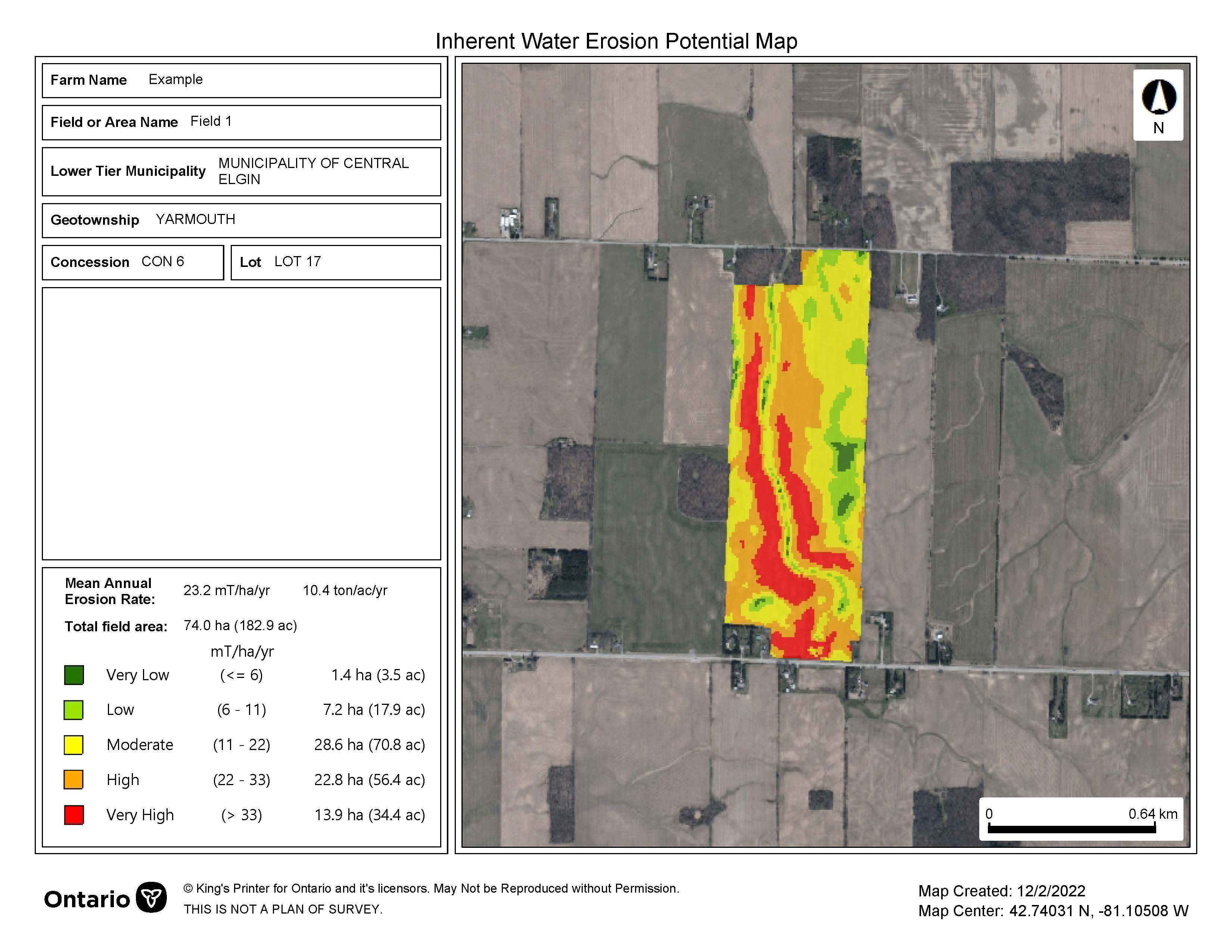
Finally, to further aid in characterizing the range of slopes and pathways present in any field where soil mapping exists in Ontario, OMAFRA has developed an online erosion risk mapping tool in AgMaps. This method offers a digital gridded approach for estimating the USLE slope length and slope gradient factors using available topographic mapping for the province. This tool can be found in the “Create Map” section of the AgMaps “Markup and Printing “ tab. Figure 8 gives an example of the type of output to expect when estimating the erosion potential across a field with varying topography. The map shows the variability of sheet and rill water erosion potential due to changes in soil characteristics and topography across the field.

Note the concentrated flow path that runs through the middle of this example field. While this feature of the field is likely to be susceptible to and experience gully erosion, the mapping does not show the area as having high sheet and rill erosion potential. The steeper side slopes, however, that direct runoff towards this central flow path do have a high potential to experience soil losses due to sheet and rill erosion.

Conclusion

This fact sheet provides guidance on how tools like the USLE and RUSLE2 are used to define:

• field slopes
• where a hillside slope starts and ends
• ways to measure the slope length and slope gradient of a field

The difference between how the USLE/RUSLE2 define slopes and flow pathways and how Ontario’s nutrient management regulation defines these terms was also described.

Even with practice and experience, no two people will arrive at the same measurements for slope length and gradient for a field because of the complexity of field topography. With experience and knowledge, however, the values different individuals choose should result in long-term average soil loss estimates that are similar in magnitude.

The online water potential mapping tool available in AgMaps can help provide further consistency in mapping the erosion potential of fields across the province.

Resources

United States Department of Agriculture — Agricultural Research Service. 2008. User’s Reference Guide — Revised Universal Soil Loss Equation Version 2 (Draft). Washington D.C.

This fact sheet was updated by Kevin McKague, P. Eng., water quality engineer, OMAFRA.