Technical appendix: Projecting Ontario’s Infrastructure Needs

Looking into the future — research and analytical tools

This chapter describes some of the tools that the government has developed to project future infrastructure needs, and it describes some of the research and analysis that the government has under consideration to further inform infrastructure decisions.

The fiscal impact of provincial infrastructure assets

As mentioned previously, the Province owns or consolidates approximately $209 billion (replacement value) in infrastructure assets, representing nearly 40 per cent of the public infrastructure stock in Ontario. Since most of our infrastructure remains in use for many years, the decisions made today have long-term impacts. Through amortization, existing provincial public infrastructure continues to have a fiscal impact^{footnote 51[51]}for decades. Given the scale involved, strong evidence is needed to ensure the right infrastructure is built in the right place at the right time.

The macro and micro context of infrastructure planning

The Ministry of Infrastructure uses a variety of analytical tools to support evidence--based decision-making. One tool is a simulation platform that analyzes infrastructure investment scenarios to determine potential infrastructure investment needs by sector and compares the differences in economic impact, costs and asset condition. It can also be used as one potential tool to consider trade-offs between sectors or between renewal and expansion investment needs within a sector.

The platform has been designed to be flexible and simulate a wide variety of scenarios. The platform is part of the ministry’s strategy to explore a range of approaches that can contribute to a better understanding of options to manage public assets. For instance, the platform can produce forecasts to show the long-term implications of different investment scenarios for asset condition. The example scenario shown in this section is illustrative and helpful in informing future approaches.

The platform has three component models:

• Stable State determines how much capital investment is needed to maintain the current level of infrastructure stock per capita through the renewal of existing assets and expansion to meet demographic growth.
• Efficient Allocation allocates infrastructure investments in sectors that have the highest marginal returns on GDP.
• Optimal estimates the level of investment in public infrastructure required to maximize long-term economic output (GDP).

Although all three models are undergoing continuous development, the Stable State model is the most advanced in terms of its methodological development and quality of input data. The Efficient Allocation and Optimal models are at a research-and-development stage, with effort being applied to understanding the sensitivity of model parameters and underlying assumptions. As a result, this section focuses exclusively on the Stable State model.

Stable State model

The Stable State model is one tool to guide evidence-based infrastructure planning and to understand the long-term implications of the investments that we make today. It uses a primarily bottom-up approach to forecast aggregate infrastructure investment needs by type and sector, while considering factors such as cost, asset condition and demographics. It is a useful model, comparing the outcomes of infrastructure choices at the aggregate level and providing overall guidance and context to future project decision making.

The Stable State model helps inform the province’s future infrastructure investment needs by sector. It does this by estimating the investment required to maintain the current infrastructure stock per capita, where stock is a proxy for the level of service that infrastructure provides to Ontarians. This is not to suggest that the current stock is necessarily appropriate in all circumstances. Rather, it provides an objective base against which we can measure the level of infrastructure investment over time. The model accomplishes this by considering the change in the mix of assets, their deterioration in condition over time and the growth in the relevant demographic for each sector. For example, for the education sector, the growth in the school-aged population is considered.

The Stable State model seeks to answer the following types of questions:

• How much investment is required to maintain infrastructure stock per capita?
• What are the long-term consequences of planned infrastructure investments on asset conditions and renewal and expansion investment needs?
• How much should the Province spend on renewal?
• How large is the renewal backlog by sector and how does this change, based on specific investment allocations?

In order to predict future investment requirements, assets are assumed to deteriorate over their useful lives along condition curves, such as the illustrative curve shown in Figure 15. Note that the model includes only infrastructure that is owned or consolidated^{footnote 52[52]}by the Province.

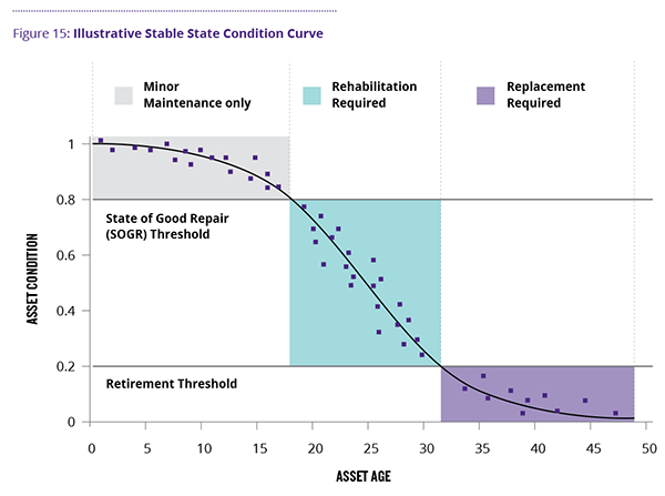
The dots on Figure 15 depict asset conditions deteriorating over time if renewal investments are not made to keep an asset in a state of good repair, with the fitted line showing the average deterioration for that asset class over time. Assets in the area above the State of Good Repair (SOGR) threshold do not require capital rehabilitation. Assets below the retirement threshold can no longer deliver service adequately and must be replaced in the near future. Lastly, although not shown in Figure 15, a maximum service life assumption is applied. In the model, each sector and asset class has its own average condition curve, as well as condition thresholds and maximum service lives. If an asset’s condition falls below the retirement threshold, or it is older than the maximum service life, the asset will need to be retired and replaced.

Within the model and at a macro level, the infrastructure needs are addressed by three categories of investment type: asset replacement, asset rehabilitation and new asset expansion to meet demographic growth.

Replacement

Assets with conditions at or below the retirement threshold or those that are older than the maximum service life limit are considered for replacement investments first, with assets in the worst condition given priority. The investment required to replace the asset is the CRV.

Rehabilitation

Assets with conditions less than SOGR, but greater than the retirement threshold, and that have not reached their maximum useful life are considered for rehabilitation investment, with assets in worse condition given priority. The timing, cost and condition effects of rehabilitation investments vary across sectors and provide an active area for investigation. The current approach generally assumes that assets are rehabilitated back to a state of good repair (rather than “new” condition) at a cost proportional to the change in condition. This rule changes for assets near the end of their service lives, where rehabilitation is only enough to extend their service life to the maximum.

Expansion to meet demographic growth

Expansion investment considers demographic trends and forecasts to estimate how much investment will be required to maintain the stock per capita in the future. Expansion requirements are determined using relevant forecasts of demographic-growth. Again, a change in the population of school-age children would drive education investments.

Accounting for infrastructure productivity

Productivity growth occurs, in infrastructure terms, when the same or more services can be provided using fewer resources. For example, incentives for off-peak travel could lead to a change in travel behaviour that ultimately increases the overall productivity of roads in congested areas. While the model has been built to allow for assumptions in productivity growth, research to implement this functionality is still at a preliminary stage.

With no productivity change, there will be a 1 per cent increase in the required amount of capital stock for every 1 per cent increase in demand (as estimated by population growth in the relevant demographic). If, instead, there is infrastructure productivity growth, the required amount of capital stock will need to grow at a slower rate than the rate of increase in demand, allowing the Province to meet a given level of demand at a lower cost to taxpayers.

Applying the Stable State model

The Stable State model has been designed to be flexible, allowing for scenarios that consider combinations of fixed-plan allocations and model-determined investments. What follows are example results for one scenario. As noted, the model is undergoing continuous improvement, with results being updated accordingly. The current model is an illustration of different macro and other tools the Ministry of Infrastructure is developing to help provide an holistic picture of public infrastructure investment needs.

Figure 16 shows the results of a scenario in which infrastructure investments reflect the Province’s10-year capital plan between 2017 and 2026 (the left half of Figure 16). In this period, the capital plan specifies the sector and asset class allocation, as well as the splits between repair and expansion investments. In the next 10 years (between 2027 and 2036), the model determines the mix of sector-level rehabilitation, renewal and expansion for demographic-growth investments required to maintain infrastructure stock per capita at 2026 levels. The result is a forecast of investment required to address service needs and provide cost-effective asset management. Results are shown in current (nominal) dollars.

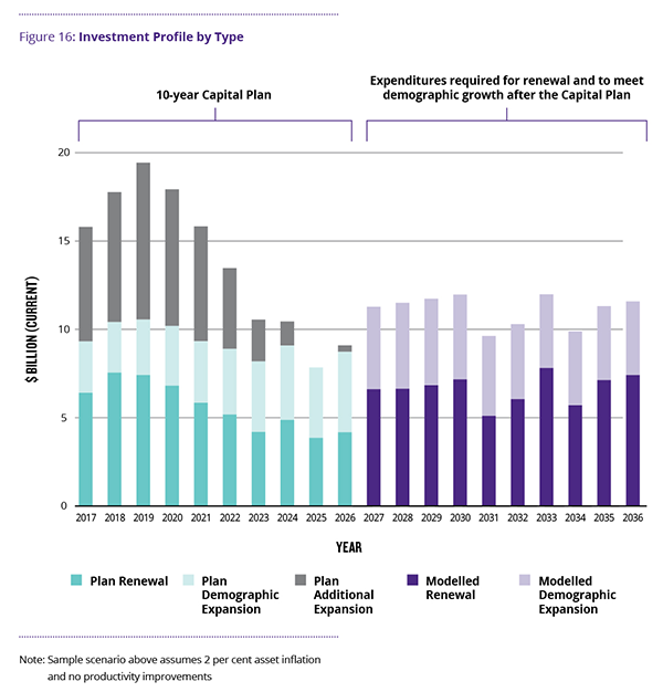
Note: Sample scenario above assumes 2 per cent asset inflation and no productivity improvements.

The preliminary results in Figure 16 suggest that there will need to be an increase (relative to the latter years of the 10-year capital plan) in the amount of renewal and rehabilitation expenditures in years 11 through 20 (2027-2036), as the Province continues to build up its infrastructure stock. There will also need to be continued expansion investment to meet demographic growth. Additional expansion (expansion that exceeds demographic growth) amounts are not projected in the years beyond the 10-year capital plan.

The model can also estimate the current and future renewal backlog. The renewal backlog is the investment needed to bring owned assets eligible for rehabilitation up to a state of good repair and to replace assets that have fallen below their retirement threshold in prior periods. In any given year, we would expect that there would be some level of renewal backlog as assets continue to age. Supported by the significant investments in renewal that are included in the 10-year capital plan, the model projects the renewal backlog to decline from 8 per cent to less than 4 per cent of the replacement value of all provincial infrastructure.

Looking into the future — strengthening data and information analysis

As discussed throughout this Technical Appendix, the Ministry of Infrastructure has made significant strides in the use of data and analysis (through the Provincial Asset Inventory and macroeconomic models) to inform the Province’s infrastructure planning. This section describes some of the next steps in the research that the ministry is considering to inform infrastructure planning. Specifically, this section discusses the need for additional data and analysis related to infrastructure capacity, demand and utilization.

The need for capacity, demand and utilization data and analysis

The ultimate purpose of Ontario’s infrastructure assets is to provide services that will benefit Ontarians. However, infrastructure assets are not homogenous. Even within asset classes, there are significant differences in capacity and demand, which consequently result in variances in the benefits that are generated from different infrastructure investments.

In order to ensure that Ontario is investing in the right infrastructure, at the right time and in the right place, it is important to understand the capacity and demand perspectives regarding infrastructure services. This involves answering questions such as: What is the capacity of our current infrastructure? How is that capacity utilized? How might demand grow in the future? What are the consequences of not meeting that demand?

These are challenging questions. The Ministry of Infrastructure is examining ways to identify, collect and analyze capacity and demand data to gain a better understanding of the utilization of public infrastructure into the future.

Infrastructure capacity

Some of the ongoing research already described in this Technical Appendix (e.g., the Provincial Asset Inventory and the Stable State model) implicitly attempts to address the question of infrastructure capacity. The general assumption behind this is that the stock of public assets (by replacement value) is a proxy for our infrastructure’s capacity to deliver related services. However, infrastructure capacity varies by time and location, due to proximity to residential and employment populations, changes in technology, synergies with other infrastructure and many other factors.

To gain a better understanding of the capacity of the Province’s current infrastructure, the Ministry of Infrastructure will be conducting research to improve the understanding of how different sectors measure capacity and how that capacity varies, or will vary, by time and location.

Infrastructure demand

As noted in the discussion of the ministry’s Stable State model, it is assumed that the demand for infrastructure services will grow with demographic growth. In general, this is true. However, growth in demand can vary due to a variety of factors, such as the prices of services and technological innovation.

As a starting point, the Ministry of Infrastructure will review the potential for collecting existing demand side/usage data and identifying gaps in demand-side data. Examples of existing demand-side data (among others) are:

• road and highway volumes
• transit ridership (passengers and passenger-kilometres)
• energy consumption
• water consumption
• hospital visits
• student populations

Infrastructure utilization

A better understanding of infrastructure capacity and demand can lead to an understanding of infrastructure utilization across sectors. Further, an understanding of demand-growth projections from ministries can help to inform the understanding of expected utilization rates across sectors in the future, and will ultimately help to inform where capacity constraints, and therefore infrastructure needs, will be the greatest. If developed, these current and future sector-wide capacity and demand metrics can ultimately be used to help inform prioritization across sectors.

Investing in the right assets, in the right place and at the right time

Capacity, demand and utilization rates across sectors may seem too dissimilar to make comparisons. However, there are steps that can be taken to quantify these factors across sectors. The Ministry of Infrastructure’s investigation in this area can provide, at the very least, some better evidence to inform cross-sector prioritization.

Brief examples of how new research and analysis can inform decisions about investing in the right infrastructure assets in the right place and at the right time are discussed below.

The right assets

Demand side/usage data matched with capacity (supply-side data) can help to inform infrastructure needs.

For example, a large increase in transit passengers indicates that the demand for transit services is increasing. Without an increase in transit capacity, service levels will drop.

Or, if demographics indicate that there will be a surge in school-aged children in certain areas, then this indicates a growing need for school capacity.

However, we cannot necessarily take for granted that past trends are indications of growth in the future. For instance, demand for transit and road use may vary with changes in land use; the distribution of residential and employment populations; new technologies; pricing; and a variety of other factors. As another example, demand for hospital visits will vary with changes in population health and the types of services that are offered in or outside of hospitals.

Seemingly unrelated factors can also affect hospital demand. For example, nearly 50,000 people were injured in road-vehicle collisions in Ontario in 2016.^{footnote 53[53]}As most vehicle collisions are caused by human error, widespread adoption of automated vehicles has the potential to eliminate the vast majority of those injuries. If this were to happen, demand for hospital visits would decrease from its baseline projection.

We should also not assume that demand growth must be met with capacity growth. Using assets more efficiently can increase the amount of service provided for a given amount of infrastructure capital. A classic example is in the case of road infrastructure, where shifting volumes to off-peak times or increasing the number of occupants per vehicle during peak hours can significantly increase the volume of passengers who travel per day — with the same amount of road capacity. The proliferation of new technologies such as ride-sharing applications has the potential to take advantage of the untapped capacity of our roads and to save money on public infrastructure. Indeed, by one estimate, the present value of potential savings created by a relatively small increase in auto occupancy rates in the Greater Toronto Area is in the range of $9 billion.^{footnote 54[54]}

Similarly, there is potential to take advantage of existing transit capacity through a variety of strategies, such as changes in the way transit services are priced (e.g., implementing peak/off-peak pricing) and by encouraging densification near existing rapid transit nodes. The ministry’s research will explore where, and how large, some of this potential is.

The right place

As noted, in much of the current thinking around infrastructure investment, there is an implicit assumption that the stock of infrastructure (denominated, for example, in current dollars) within a given sector is a proxy for infrastructure capacity. Perhaps, as a very general rule, this is true. Nevertheless, it is undeniable that, for a given amount of infrastructure stock, either within or across sectors, there can be large variations in the capacity that the stock can deliver. This is especially true when considering the location of infrastructure assets and the proximity of the services that they provide relative to the proximity of their users (i.e., individuals and businesses).

An example — courtroom capacity

An example that illustrates the above point is the capacity of Ontario’s courtrooms. Collectively, Ontario’s courtrooms may have capacity that is greater than the number of current or even projected cases. Yet, at the local level, there are observed instances where the current courthouse is at or above capacity today, and this overcapacity would continue to grow if the trend continues.

By using the province-wide measure of capacity, few or no new courthouses would be built, forcing residents in newly developed areas to travel long distances to the nearest existing courthouse with capacity. On the other hand, building and maintaining new courthouses wherever there is demand at the local subdivision level is extraordinarily expensive. Clearly, there is a balance to be achieved that trades off access costs for residents against capital and operating costs.

This balance is not unique to courthouses, of course. It also applies to hospitals, schools, recreational facilities and other kinds of assets.

Capacity metrics

All sectors implicitly make some trade-offs between access time and capital costs when defining infrastructure needs. The Ministry of Infrastructure is designing research to help make those trade-offs more explicit. For instance, it is conceivable that province-wide capacity in each sector can be defined according to different access-time thresholds.

It may be difficult to evaluate gains as a result of improvements in access times for residents^{footnote 55[55]}. However, the cost of providing the necessary infrastructure to achieve the same level of capacity at different access-time thresholds can be calculated. For example, to provide the same amount of capacity at a maximum access time of one hour might cost $100 million more annually than to provide the same capacity at a maximum access time of 1.5 hours. We can then ask, “Is it advantageous overall to spend $100 million annually to decrease maximum access times by 30 minutes?”

These metrics can be analyzed across the Province’s entire portfolio of infrastructure assets. Analysis of this nature might entail exploring questions such as: “Would $1 billion spent to reduce hospital access times be a better investment than reducing access times to schools or parks?”

The role of transportation

New roads, bridges, and transit systems or, alternatively, more efficient use and operation of those assets, can improve access times to all infrastructure assets. Transportation investments, then, can increase province-wide capacity in the various sectors. However, it is important that these transportation investments are made in the right place, relative not only to other existing public infrastructure, but also to existing and future residential and employment populations and key attractions. As with other types of infrastructure, it is also important that we make the best and most-efficient use of existing transportation infrastructure before adding new infrastructure.

The right time

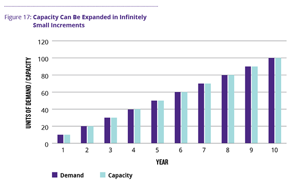
In general, there is a “lumpiness” to infrastructure capacity. In more technical terms, this means that infrastructure capacity cannot be added in infinitely small increments. This lumpiness poses a problem for capacity expansions. If capacity is always added before utilization is at 100 per cent, there will always be wasted capacity (tying up capital that could be employed elsewhere in the public sector or broader economy). On the other hand, if capacity is always added after utilization is at 100 per cent, service levels will drop and some potential users will be left without service. This problem is exacerbated by long planning and construction lead times associated with adding capacity (more so for some investments than others).

Take for example an “ideal” situation, in which capacity can be added in infinitely small increments. Figure 17 shows this situation over a 10-year period, where both demand and capacity increase by 10 units each year. The result is that demand is always equal to capacity, leaving no excess demand or excess capacity.

What if we were faced with the same demand profile, but capacity could be added only in units of 50? In that situation, we would be left with a trade-off between excess capacity and excess demand in any given year.

The trade-off that we ultimately choose depends on the relative costs of excess capacity and excess demand. If the cost of having excess demand far exceeds the cost of having excess capacity, the decision rule might be to add capacity, so that demand never exceeds capacity in any given year. Figure 18 shows this situation, using the same demand-growth profile as in Figure 17.

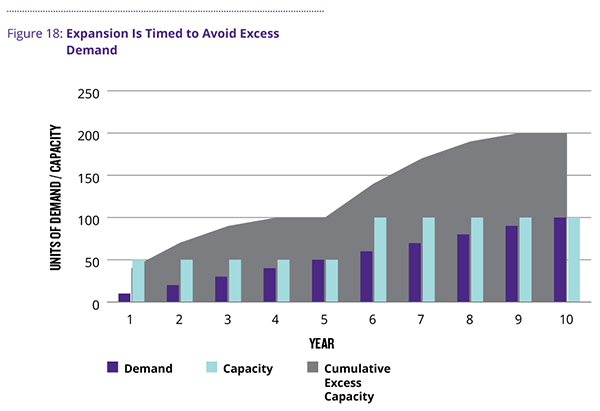
Because capacity can only be added in increments of 50 units, there is excess capacity in years one through four, and again in years six through nine. Over the 10-year period, the cumulative excess capacity is 200 units. The cost of this excess capacity is the opportunity cost of the unused capital, plus any additional maintenance and operating costs associated with running a facility that is larger than is needed at the time.

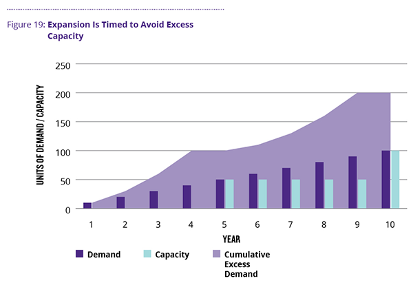
If, on the other hand, the cost of excess capacity far outweighed the cost of excess demand, the decision rule might be to time expansion of capacity so that there is never any wasted capacity. Figure 19 presents this situation.

In this case, there is excess demand in years one through four, and again in years six through nine. Over the whole period, cumulative excess demand is 200 units. The cost of this excess demand is the lost benefit that customers would have gained by having had access to the services that they wanted, or the loss in service levels.

As noted, the decision rule of when to add capacity should be informed by the relative costs of excess capacity and excess demand. In a simple situation, where the cost of one unit of excess capacity was equal to the cost of one unit of excess demand, the decision rule could be to expand capacity, so that the sum of cumulative excess capacity and cumulative excess demand was minimized. Figure 20 presents this situation.

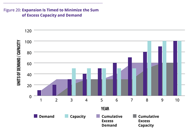
In this case, there are alternating periods of excess capacity and excess demand. Over the 10-year period, cumulative excess demand is 60 units, as is cumulative excess capacity, with the sum of the two being 120 units. Given this demand profile and the constraint that capacity can only be expanded in 50-unit increments, 120 units of cumulative excess capacity and demand is the lowest possible total.

These are, of course, simple examples. Practical, real-world models would have to consider the consequences that are specific to each investment decision, or at least specific to the broader set of assets.

Generally, the consequences of excess capacity will be somewhat common across asset classes, as long as the opportunity cost of capital is similar.

The consequences of having excess demand will vary significantly both across and within sectors. Excess demand for hospitals could mean longer wait times, increased illness and possibly increased mortality rates, among many other results. Excess demand for schools could mean suboptimal class sizes, longer than ideal travel times for some students (to travel to nearby schools with available capacity), the use of portables for temporary capacity and other measures.

Within sectors, these trade-offs are either made explicitly or implicitly. Across sectors, these trade-offs are made implicitly. To make optimal decisions across sectors, one needs a better understanding of the consequences of excess demand, based on better data and analytics.

Other factors to consider

For cross-sector prioritization, it is important to take other factors into consideration, such as the cost of being over capacity and under capacity in each sector, volatility/uncertainty in demand and whether different regions allow sharing of capacity, among many others. All these questions, however, start with the need to measure capacity, demand and utilization. Any improvement in our understanding and measurement of capacity, demand and utilization across sectors will help to inform the prioritization process, while considering other important factors for prioritization.

Infrastructure planning and prioritization

Strengthening infrastructure planning and prioritization through cross-ministry collaboration

As required under the IJPA, when evaluating infrastructure investments, the Province considers a range of evidence including the life-cycle costs of an asset, and whether a project would stimulate the economy, align with public policy goals, and achieve a long-term return on investment.

Building on the principles of the IJPA, the Ministry of Infrastructure is engaged in developing and implementing a three-year transformation plan, intended to increase the government’s capacity to make informed decisions for infrastructure investments. To prioritize projects and programs, the ministry is creating an evidence-based analytical framework to strengthen the prioritization of projects and programs that take infrastructure planning principles into account. These principles will support ministries in developing solid business cases that are comparable across sectors. This will help ministries build their capacity on infrastructure planning and project prioritization in the context of the plan.

Through cross-ministry collaboration, the government is undertaking a broad review of infrastructure planning and identifying best practices that can be implemented across Ontario’s ministries and agencies. Best practices will be reflected in guidance for ministries, which will help set standard practices for improving business cases. The guidelines will bring further consistency and transparency to the ministry’s prioritization efforts.

The Ministry of Infrastructure has outlined a three-year plan for strengthening infrastructure planning and prioritization, like the three-year timeframe for asset management:

• In 2017, the Ministry of Infrastructure is working with Treasury Board Secretariat to operationalize the first phase of an enhanced Planning and Prioritization Framework, building on the planning that ministries are currently undertaking. The framework will identify critical investments that address infrastructure needs. The Ministry of Infrastructure is also working with the Ministry of Municipal Affairs to assess the alignment of proposed infrastructure projects with municipal Official Plans as well as the province’s land-use planning framework.
• In 2018, the Planning and Prioritization Framework will continue to be enhanced. As part of this, the Ministry of Infrastructure will work with other ministries to identify and build consensus on criteria for strengthening the prioritization of infrastructure projects across sectors, and to test identified criteria. The Ministry of Infrastructure will also provide guidance to other ministries, so they can develop solid business cases, comparable across sectors, to support this prioritization. This will be aligned with the requirements for Treasury Board/Management Board of Cabinet submissions and directives. Strong business cases will strengthen ministries’ ability to identify the right investments, including assessing whether there are alternative ways of delivering services that could avoid the need to invest. Comparability across sectors will improve the integration and alignment of investments across sectors.
• In 2019, the Ministry of Infrastructure will work towards obtaining infrastructure proposals that are supported by robust and consistent business cases and assessed against common prioritization criteria, including — but not limited to — those that measure economic, social and environmental impacts. In addition, the government will strengthen the alignment of infrastructure planning and investment decisions with municipal Official Plans as well as the province’s land-use planning framework in order to improve the development of integrated, complete communities and regions.