Meteorological data and Receptor locations
6.0 Meteorological Data
Section 13 of the Regulation specifies the types of meteorological information that can be used with an approved dispersion model as follows:
Meteorological data
“13. (1) An approved dispersion model that is used for the purposes of this Part shall be used with one of the following types of meteorological information:
- Regional surface and upper air meteorological data for the part of Ontario in which the source of contaminant is located that was available on May 14, 2007, andcontinues to be available, through a website maintained by the Ministry on the internet or through the Ministry’s Public Information Centre.
1.1 Data described in paragraph 1 that has been processed by the AERMET computer program, as that program is amended from time to time,and that is available through a website maintained by the Ministry on the Internet or through the Ministry’s Public Information Centre, if the approved dispersion model that is used is the AERMOD dispersion model described in paragraph 1 of subsection 6 (1).
- Data described in paragraph 1.1 that has been refined to reflect local land use conditions, if the approved dispersion model that is used is the AERMOD dispersion model described in paragraph 1 of subsection 6 (1).
2.1 Data described in paragraph 1 that has been processed by the PCRAMMET computer program, as that program is amended from time to time, and that is available through a website maintained by the Ministry on the Internet or through the Ministry’s Public Information Centre, if the approved dispersion model that is used is the ISCPRIME dispersion model described in paragraph 3 of subsection 6 (1).
- Local or site-specific meteorological data approved by the Director as an accurate reflection of meteorological conditions.
- Data obtained from a computational method, if the Director is of the opinion that the data is at least as accurate as data that would be obtained by local or site-specific meteorological monitoring.
(2) Despite subsection (1),the Director may give written notice to a person who discharges or causes or permits the discharge of a contaminant requiring that an approved dispersion model that is used for the purposes of this Part be used with a type of meteorological information specified in the notice that, in the opinion of the Director, accurately reflects meteorological conditions.
(3) Before the Director gives a person a notice under subsection (2), the Director shall give the person a draft of the notice and an opportunity to make written submissions to the Director during the period that ends 30 days after the draft is given.
(4) This section does not apply if the approved dispersion model that is used is,
- the ASHRAE method of calculation;
- the SCREEN3 dispersion model described in paragraph 4 of subsection 6 (1);
- the method of calculation required by the Appendix to Regulation 346; or
- a dispersion model or combination of dispersion models that, pursuant to subsection 7 (3), is deemed to be included in references in this Part to approved dispersion models, if the dispersion model or combination of dispersion models is not capable of using meteorological data.
6.1 Comparison of SCREEN3 with AERMOD Model Requirements
Meteorological data is essential for air dispersion modelling as it describes the primary environment through which the contaminants being studied migrate. Similar to other data requirements, screening model requirements are less demanding than the more advanced models.
SCREEN3 provides three methods of defining meteorological conditions without using actual meteorological data or measurements. These are as follows:
- Full Meteorology: SCREEN3 will examine all six stability classes (five for urban sources) and their associated wind speeds. SCREEN3 examines a range of stability classes and wind speeds to identify the "worst case" meteorological conditions, i.e., the combination of wind speed and stability that results in the maximum concentrations.
- Single Stability Class: The modeller can select the stability class to be used (A through F). SCREEN3 will then examine a range of wind speeds for that stability class only.
- Single Stability Class and Wind Speed: The modeller can select the stability class and input the 10-metre wind speed to be used. SCREEN3 will examine only that particular stability class and wind speed.
Note that modellers should select the “full meteorology” option when using SCREEN 3 to assess POI concentrations under the Regulation.
6.2 Preparing Meteorological Data for use with AERMOD Dispersion Modelling
AERMOD requires actual hourly meteorological conditions as inputs. This model requires pre-processed meteorological data that contains information on surface characteristics and upper air definition. This data is typically provided in a raw or partially processed format that requires processing through a meteorological pre-processor. AERMOD uses a pre-processor known as AERMET which is described further below.
6.2.1 Hourly Surface Data
Hourly surface data is supported in several formats including the CD-144 file format, the SCRAM surface data file format, the ISHD format (TD-3505), and SAMSON surface data as shown below.
- CD-144 – NCDC Surface Data: This file is composed of one record per hour, with all weather elements reported in an 80-column card image. Table 6-1 lists the data contained in the CD-144 file format that is needed to pre-process your meteorological data.
Table 6-1: CD-144 Surface Data Record (80 Byte Record) Element Columns Surface Station Number 1-5 Year 6-7 Month 8-9 Day 10-11 Hour 12-13 Ceiling Height (Hundreds of Feet) 14-16 Wind Direction (Tens of Degrees) 39-40 Wind Speed (Knots) 41-42 Dry Bulb Temperature (°Fahrenheit) 47-49 Opaque Cloud Cover 79 - MET-144 – SCRAM Surface Data: The SCRAM surface data format is a reduced version of the CD-144 data with fewer weather variables (28-character record). Table 6-2 lists the data contained in the SCRAM file format.
Table 6-2: SCRAM Surface Data Record (28 Byte Record) Element Columns Surface Station Number 1-5 Year 6-7 Month 8-9 Day 10-11 Hour 12-13 Ceiling Height (Hundreds of Feet) 14-16 Wind Direction (Tens of Degrees) 17-18 Wind Speed (Knots) 19-21 Dry Bulb Temperature (° Fahrenheit) 22-24 Total Cloud Cover (Tens of Percent) 25-26 Opaque Cloud Cover (Tens of Percent) 27-28 SCRAM is an older format developed by the US EPA specifically for use by air dispersion models. It does not contain several weather variables, which are necessary for dry and wet particle deposition analysis, including:
- Surface pressure: for dry and wet particle deposition;
- Precipitation type: for wet particle deposition only; or
- Precipitation amount: for wet particle deposition only.
- SAMSON Surface Data: The SAMSON data format contains all of the required meteorological variables for concentration, dry and wet particle deposition, and wet vapour deposition. The SAMSON data elements used by AERMET and the corresponding Element IDs are shown below in Table 6-3.
Table 6-3: SAMSON Surface Data Elements Element Element ID Total cloud cover 6 Opaque cloud cover 7 Dry bulb temperature 8 Relative humidity 10 Station pressure 11 Wind direction 12 Wind speed 13 Ceiling height 15 Hourly precipitation amount and flag 21 - Integrated Surface Hourly Data (ISHD): Data in this format, which is supported by the US EPA, is available for download from the US National Oceanic and Atmospheric Administration (NOAA), and is in the TD-3505 format. It contains a large number of data elements, many of which are not used by AERMET. Note that ISHD data is reported in Greenwich Mean Time (GMT).
If the processing of raw data is necessary, the surface data must be in one of the above formats in order to successfully pre-process the data using AERMET. Canadian hourly surface data can be obtained from Environment Canada, or US NOAA. Regional pre-processed meteorological data sets can be obtained from the Public Information Centre [Ontario Regional Meteorological Data (PIBs # 5081e01)] or the Map: Regional Meteorological and Terrain Data for Air Dispersion Modelling website.
6.2.2 Upper Air Data
AERMET requires the full upper air sounding data. These data for the Ontario regions are available from the Public Information Centre [Ontario Regional Meteorological Data (PIBs # 5081e01)] or the Map: Regional Meteorological and Terrain Data for Air Dispersion Modelling website.
Subject to ministry approval under section 13, other upper air data can be used; for example:
- observations (i.e. upper air soundings) from other stations, or
- data generated from mesoscale meteorological models, such as the North America Model (NAM) or North America Regional Reanalysis (NARR)
6.2.3 AERMET and the AERMOD Model
The AERMET program is a meteorological pre-processor which prepares hourly surface data and upper air data for use in the US EPA air quality dispersion model AERMOD. AERMET was designed to allow for future enhancements to process other types of data and to compute boundary layer parameters with different algorithms.
AERMET processes meteorological data in three stages:
- The first stage (Stage 1) extracts meteorological data from archive data files and processes the data through various quality assessment checks.
- The second stage (Stage 2) merges all data available (surface data, upper air data, and on-site data) and stores these data from all hours together in a single file.
- The third stage (Stage 3) reads the merged meteorological data along with the land use surface characteristics (Chapter 5.4) to estimate the necessary boundary layer parameters for use by AERMOD.
Out of this process two files are written for AERMOD:
- A Surface File of hourly boundary layer parameters estimates; and
- A Profile File of multiple-level observations of wind speed, wind direction, temperature, and standard deviation of the fluctuating wind components.
6.3 Regional Meteorological Data
The ministry has prepared regional meteorological data sets for use in Tier 2 modelling using AERMOD. These are standard data sets that can be used for air quality studies using AERMOD.
For AERMOD, the meteorological data sets are available in two formats:
- Regional model ready data for AERMOD, with land characteristics for crop, rural and urban conditions.
- Regional pre-processed hourly surface data and upper air data files ready for AERMET (stages 1, 2 and 3), which allows consideration of site-specific local land use conditions.
The above data sets are available from the Map: Regional Meteorological and Terrain Data for Air Dispersion Modelling website, and provide a unique, easily accessible resource for air dispersion modellers in the province of Ontario (see section 13 of the Regulation). The availability of standard meteorological data reduces inconsistencies in data quality and requests to the ministry for meteorological data sets. The regional data sets shall not be modified when used for the purpose of paragraph 1 of subsection 13 (1) of the Regulation. If the pre-processed data sets are used with site-specific land use conditions as per paragraph 2 of subsection 13 (1), this must be documented in the submission as per paragraph 10 of subsection 26 (1) of the Regulation and it is strongly recommended that modellers consult EMRB for guidance or review prior to the completion of model runs.
Each regional data set was developed using surface and upper air data from the nearest representative meteorological station. The surface meteorological sites used were Toronto (Pearson Airport), London, Sudbury and Ottawa along with International Falls, MN and Massena, NY. Note in Table 6-4 there exist two ID numbers for Massena and International Falls. The ID within brackets represents the United States System while the other is the ID for the International System. The following meteorological elements were used in AERMET processing for the 5 year period:
- ceiling height;
- wind speed;
- wind direction;
- air temperature;
- total cloud opacity; and
- total cloud amount.
The upper air stations used were Maniwaki, QC, White Lake, MI, Buffalo, NY, Albany, NY and International Falls, MN. Table 6-4 gives the locations of the surface meteorological sites and lists the upper air station to be used for each site. The locations of the upper air sites are given in Table 6-5.
| Surface station | ID | Latitude | Longitude | Height above sea level, m | Province/State | UA to use |
|---|---|---|---|---|---|---|
| Sudbury | 6068150 | 46.62 | -80.8 | 348 | ON | White Lake |
| Ottawa | 6106000 | 45.32 | -75.67 | 114 | ON | Maniwaki |
| London | 6144475 | 43.03 | -81.15 | 278 | ON | White Lake |
| Toronto | 6158733 | 43.67 | -79.6 | 173 | ON | Buffalo |
| Massena | 72622 (94725) | 44.9 | -74.9 | 65 | NY | Albany |
| International Falls | 72747 (14918) | 48.57 | -93.37 | 359 | MN | International Falls |
Note: All surface stations have an anemometer height of 10 m.
| UA station | ID | Latitude | Longitude |
|---|---|---|---|
| Buffalo | 725280 | 42.93 | -78.73 |
| Maniwaki | 7034480 | 46.23 | -77.58 |
| Albany | 725180 | 42.75 | -73.8 |
| White Lake | 726320 | 42.7 | -83.47 |
| International Falls | 727470 | 48.57 | -93.37 |
6.3.1 Regional Meteorological Data Processing Methodology
The original surface meteorological data was pre-processed by the ministry to reduce the amount of missing data and to use a minimum wind speed of about 1 m/s. Use of a 1 m/s minimum wind speed essentially eliminates missing hours due to calm conditions. A calm hour is defined as a period where the wind speed is below the measurement threshold of the anemometer. During these periods, the data is often reported as missing, since both the wind speed and direction are either non-existent or highly uncertain. Atmospheric dispersion is typically quite poor during calm conditions, which can lead to elevated pollutant concentrations in the vicinity of a facility. As a result, the ministry regional data sets were processed using a specific methodology to remove the calms and set the minimum wind speed to 1 m/s. Also, the wind directions were randomized to account for the variability in wind directions during these periods. This allows the model to calculate concentrations during these periods. The pre-processing steps were as follows:
- Treatment of Wind Speed and Direction for Calm/Missing Conditions - Data sets that had approximately 5% or more missing or calm hours, were pre-processed by first filling these missing/calm hours with data from a nearby station with similar climatology. For example, missing/calm hours in the original International Falls and Massena data sets were filled by Kenora and Dorval data, respectively. Any remaining missing/calms hours (if less than 6 consecutive hours in a row) were then interpolated as described below, and the interpolated wind directions were randomized using a random number file. Hours with calm or very low wind speeds were set to minimum speeds of 4 km/h (~1 m/s).
- Interpolation of Missing Values As indicated above, if missing hours remained after backfilling with data from another station, linear interpolation was applied to a maximum of six missing hours in a row. Note that missing data that occurred at the very beginning and at the very end of the data set (i.e., the first few hours in January of the first year of meteorological data, and the last few hours in December of the last year of meteorological data) were left as "missing", and no extrapolation was applied. Also, if the number of consecutive hours with missing values for the element was more than six, the entire block of values were left as "missing".
- Unit Conversion - All data from Canadian sites were converted to the United States standard format required for input into AERMET, as previously set out in Table 6-1 and Table 6-2.
The AERMOD ready regional meteorological data sets were generated by the 3 stage AERMET process for three different wind independent surface categories, called “urban”, “forest” and “crops”. These three categories/files allow users to choose the file that most accurately reflects the land use conditions in the vicinity of their site. For each of these three surface types, the ministry used a weighted-average of surface parameters for the typical mix of land uses seen in Ontario for each land use class considered in the category. For example, the surface characteristics in the forest regional data sets were calculated assuming that typical forests in Ontario are comprised of a mix of 50% deciduous and 50% coniferous trees.
As indicated previously, the surface characteristics that are adjusted to reflect land use conditions are the albedo (A), the Bowen ratio (Bo) and the surface roughness (Zo). The parameter values used in each of the AERMOD ready regional files were derived from data in Tables 4.1, 4.2b (albedo for average conditions) and 4.3 of the AERMET User’s Guide(8) and the weightings of different land uses considered in each file. These are shown in Table 6-6, Table 6-7 and Table 6-8 below for each category/file.
“urban” – all surface parameters were set to urban values, as in Table 6-6.
| Season | A | Bo | Zo |
|---|---|---|---|
| Winter | 0.35 | 1.5 | 1 |
| Spring | 0.14 | 1 | 1 |
| Summer | 0.16 | 2 | 1 |
| Fall | 0.18 | 2 | 1 |
“forest” – all surface parameters were set to the mixture of coniferous and deciduous forests in the ratio 50%/50% as in Table 6-6.
| Season | A | Bo | Zo |
|---|---|---|---|
| Winter | 0.42 | 1.5 | 0.9 |
| Spring | 0.12 | 0.7 | 1.15 |
| Summer | 0.12 | 0.3 | 1.3 |
| Fall | 0.2 | 0.9 | 1.05 |
“crops” – all surface parameters were set to the mixture of Grassland, Cultivated Land, and Coniferous and Deciduous forest in the ratio: 45%/45%/5%/5% as in Table 6-7.
| Season | A | Bo | Zo |
|---|---|---|---|
| Winter | 0.6 | 1.5 | 0.095 |
| Spring | 0.16 | 0.35 | 0.15 |
| Summer | 0.19 | 0.65 | 0.265 |
| Fall | 0.19 | 0.85 | 0.13 |
These AERMOD-ready files may be used if the surface characteristics for a radius of 3 km around the facility are reasonably represented by the surface characteristics of one of the prepared files. Note that the values in the above tables are somewhat different than those presented earlier in Table 5-1 to Table 5-3, which were derived from information presented in the AERSURFACE User’s Guide. The values in AERSURFACE represent a refinement over those in AERMET as there are 21 land use categories in comparison to the 8 in AERMET. The AERSURFACE data can be used in the development of local meteorological data sets where more detail may be necessary to accurately specify the land use patterns in the area. However, the regional meteorological data sets are intended to be somewhat generic, for use at a variety of locations in each region. As a result, ministry considers the use of the AERMET values in the regional data sets to be valid and representative.
In cases where the surface characteristics at a site do not reasonably match those defined in any of the AERMOD-ready regional meteorological data sets, for example when there are significant areas of water coverage within a 3 km radius, paragraph 2 of subsection 13 (1) of the Regulation allows a modeller to use site-specific surface conditions (i.e. local land use) in combination with the ministry’s pre-processed surface and upper air data files in a Tier 2 assessment. In the Stage 3 processing of the meteorological data with AERMET, different surface characteristics may be entered on a variable sector size basis. The surface characteristics for each sector must be the weighted average for a radius of 3 km from the facility. The choice of surface characteristics (surrounding land use) must be well documented and provided as part of a modeller’s submission (paragraph 10 of subsection 26 (1) of the Regulation). It is strongly recommended that modellers pre-consult ministry (EMRB) if values for the surface characteristics other than those set out previously in Table 5-1 to Table 5-3 are proposed for use.
6.3.2 Use of Ministry Regional Meteorological Data
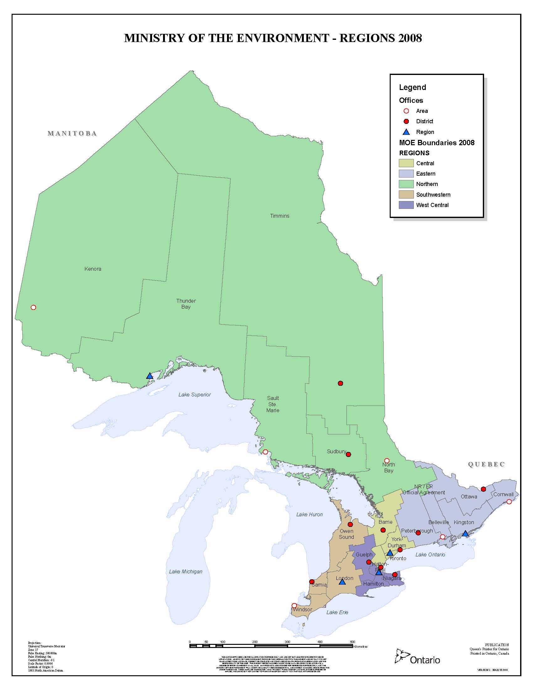
The application of the regional meteorological data sets across Ontario is described in Table 6-9. This table lists the ministry region and districts for which each of the meteorological data sets is most applicable. A map of the districts can be found in Figure 6.1.
| Meteorological Data Set | Ministry Region | Ministry District/Area |
|---|---|---|
| Toronto | Central | Toronto, York-Durham,Halton-Peel, Barrie, Owen Sound |
| London | Southwestern | London, Windsor, Sarnia |
| London | West Central | Hamilton, Niagara, Guelph |
| Ottawa | Eastern | Ottawa, Peterborough, Belleville |
| Sudbury | Northern | Sudbury, North Bay, Sault Ste. Marie, Timmins |
| International Falls | Northern | Thunder Bay, Kenora |
| Massena | Eastern | Kingston, Cornwall |
Figure 6.1: Ontario Ministry of Environment and Climate Change Regions and Their Offices
6.4 Local and Site-Specific Meteorological Data
Meteorological data quality is of critical importance, particularly for reliable air dispersion modelling using models such as AERMOD. If data other than the ministry’s Regional Meteorological data sets are used in air dispersion modelling assessments, careful quality control must be used throughout the entire processing phase to ensure that the data set is complete and representative of the site being modelled.
There are four factors that affect the representativeness of the meteorological data. These are: 1) the proximity of the meteorological site to the area being modelled; 2) the complexity of the terrain; 3) the exposure of the meteorological measurement site; and 4) the time period of the data collection. It should be emphasized that representativeness (both spatial and temporal) of the data is the key requirement. One factor alone should not be the basis for deciding on the representativeness of the data.
The meteorological data that is input to a model must be selected based on its appropriateness for the modelling project. More specifically, local meteorological data must be representative of the wind flow in the specific area being modelled, so that it properly represents the transport and diffusion of the contaminants being modelled.
As indicated earlier, no approval is required to use the appropriate regional meteorological data set. However, during the assessment it may be determined that the regional meteorological data sets are not representative of the meteorology at the location of the facility. This may be the case where there are differing dominant land uses or terrain in the vicinity that are not captured in the regional met data sets, such as those located next to significant terrain features or large water bodies. In these situations, use of a local data set would be more representative.
Note that ministry approval must be obtained to use any local or site-specific meteorological data set (see paragraphs 3 and 4 of subsection 13 (1) of the Regulation). In some cases, a modeller may be required
6.4.1 Expectations for Local Meteorological Data Use
Pre-processed, AERMOD-ready local surface and upper air data files may be obtained from the ministry upon request. Alternately, raw meteorological data may be obtained from Environment Canada, on-site meteorological stations
When using any data sets that are not processed by the ministry, the quality of the data, origin of the data and any processing applied to the raw data must be outlined for review by the ministry. Missing meteorological data and calm wind conditions can be handled in an approach similar to that used for the generation of the regional meteorological data sets (described in Chapter 6.3.1). Modellers who wish to or who are required to use local or site-specific meteorological data must obtain pre-approval by the ministry by completing a subsection 13 (1) request form, prior to the submission of an ESDM report.
When Environment Canada sites are used as the source of local met data, the ministry requires a description of why the Environment Canada site is representative for the facility and an assessment of the completeness of the data set. This information must be reviewed by the ministry before the modeller develops and processes the local meteorological data set, otherwise approval may not be granted.
When on-site meteorological data is used, the sources of all of the data used to produce the meteorological file, including cloud data and upper air data must be documented. The modeller also needs to:
- describe why the site chosen is representative for the modelling assessment;
- describe the Quality Assurance and Quality Control (QA/QC) program for the station, and the date of last calibration;
- include a description of any topographic impacts or impacts from obstructions (trees, buildings etc.) on the wind monitor;
- supply information on the monitoring equipment, and the height(s) that the wind is measured;
- supply the time period of the measurements (measurement interval, recording interval, averaging period and method (vector or scalar)); and
- supply the data completeness and the percentage of calm winds.
In preparing regional meteorological data sets, the ministry treated calms winds and missing data as described in Chapter 6.3.1. A similar discussion of the data QA/QC methodology must be presented when modellers process local meteorological data for approval, along with the treatment of calm wind and missing data.
Wind roses showing the wind speed and directions shall be provided with the modelling assessment. If wind direction dependent land use was used in deriving the final meteorological file, the selection of the land use shall be documented as per paragraph 10 of subsection 26 (1) of the Regulation.
Use of computationally generated local meteorological data with WRF or another meteorological model is an extremely complex process, with many data inputs and QA/QC requirements. Modellers who choose to use this approach are strongly encouraged to preconsult with EMRB for guidance in advance of running the meteorological model, otherwise approval under subsection 13 (1) may not be granted.
6.5 Elimination of Meteorological Anomalies
In modelling applications using regional or local meteorological data sets, certain extreme, rare and transient metrological conditions may be present in the data sets that may be considered outliers. As such, for assessments of 24-hour average concentrations, the highest 24-hour average predicted concentration in each single meteorological year may be discarded, and the ministry will consider for compliance assessment the highest concentration after elimination of these five 24-hour average concentrations over the 5-year period from the modelling results. In assessments of annual concentrations, the highest annual concentration in the 5-year period will be considered, without removal of any meteorological anomalies.
For shorter averaging periods, such as 1-hour concentrations, the eight hours with the highest 1-hour average predicted concentrations in each single meteorological year may be discarded. The ministry will consider for compliance assessment the highest concentration after elimination of these forty hours over the five-year period from the modelling results. This approach is for modelling results only (i.e. models with meteorological data inputs) and does not apply to measured or monitored concentrations. Note that the elimination of these anomalies is optional. Results will always be conservative if the meteorological anomalies are not eliminated.
Although some commercially available modelling software packages will select these values automatically, it can be done manually. If modelling using AERMOD, this approach can be applied by selecting the Maximum Values Table (MAXTABLE) option in the Output Pathway. A description of how the MAXTABLE could be used to eliminate meteorological anomalies is given in Appendix B.
7.0 Receptor Locations
The AERMOD air dispersion model computes the concentrations of contaminants emitted from user-specified sources at user-defined spatial points. Modellers commonly refer to these points as receptors. These receptors are used in the modelling exercise to determine concentrations of contaminants at points of impingement as defined in section 2 of the Regulation. Proper placement of receptors is important to ensure that the location of the maximum POI concentration is determined. This can be achieved through several approaches. The types of receptors and receptor grids are described in Chapter 7.1, followed by a discussion in Chapter 7.2 on the grid extents and receptor densities required to capture maximum point of impingement concentrations as required by section 14 of the Regulation.
7.1 Receptor Types
Models such as AERMOD support a variety of receptor types that allow for considerable user control over calculating contaminant concentrations. The major receptor types and grid systems are described in the following subchapters. Further details on additional receptor types can be found in the appropriate documentation for each model.
7.1.1 Cartesian Receptor Grids
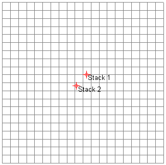
Cartesian receptor grids are receptor networks that are defined by an origin with evenly (uniform) or unevenly (non-uniform) spaced receptor points in x and y directions. Figure 7.1 illustrates a sample uniform Cartesian receptor grid.
Figure 7.1: Example of a Cartesian Grid
7.1.2 Polar Receptor Grids
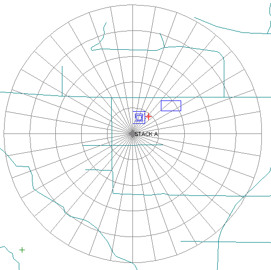
Polar receptor grids are receptor networks that are characterized by an origin with receptor points defined by the intersection of concentric rings, which have defined distances in metres from the origin, with direction radials that are separated by a specified degree spacing. Figure 7.2 illustrates a sample uniform polar receptor grid.
Figure 7.2: Example of a polar grid
7.1.3 Multi-Tier Grids
Each receptor point requires computational time. Consequently, it is not optimal to specify a dense network of receptors over a large modelling area; the computational time would negatively impact productivity and available time for proper analysis of results. An approach that combines aspects of coarse grids and refined grids in one modelling run is the multi-tier grid.
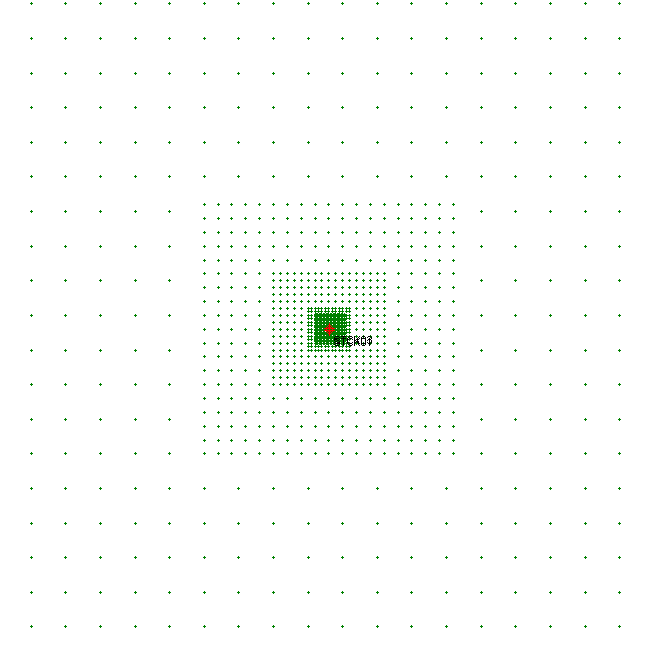
The multi-tier grid approach strives to achieve proper definition of points of maximum impact while maintaining reasonable computation times without sacrificing sufficient resolution. Figure 7.3 provides an example of a type of multi-tier grid that is required under subsection 14 (1) of the Regulation (see Chapter 7.2).
Figure 7.3: Sample Multi-Tier Grid Spacing with 5 tiers of Spacing
7.1.4 Fenceline Receptors
With the exception of same structure contamination and certain on-site receptors specified in section 2 of the Regulation, dispersion modelling for on-site receptors, or within the property boundary, is not normally required. As a result, property boundaries are typically delineated in projects and model results are not required within those areas. However, as per the requirements in subsection 14 (2), receptors must be placed along the plant boundary to demonstrate compliance at the nearest reportable geographical locations to the sources.
A receptor network based on the shape of the property boundary that has receptors parallel to the boundaries is often a good choice for receptor geometry. The receptor spacing can then progress from fine to coarse spacing as distance increases from the facility, similar to the multi-tier grid.
7.1.5 Discrete Receptors
Receptor grids do not always cover precise locations that may be of interest in modelling projects. Specific locations of concern such as a monitoring station or a residence can be modelled by placing single (discrete) receptors, or additional refined receptor grids, at desired locations. This enables the modeller to assess data on specific points for which accurate data is especially critical. In particular, concentrations of a contaminant at elevated points of impingement can be greater than concentrations found at ground level points of impingement. Depending on the project resolution and location type, elevated receptors can be characterized by discrete receptors, a series of discrete receptors, or an additional receptor grid.
Some ESDM reports such as those completed in response to a notification of a Upper Risk Threshold (URT) exceedance under section 30 of the Regulation require an assessment of concentrations at specific receptor locations. Receptors of particular interest are set out in subsection 30 (8) of the Regulation.
Under Section 30 of the Regulation – Upper Risk Thresholds:
“30 (8) The following places are the places referred to in subsection (7) and in subsection 32 (22):
- A health care facility.
- A senior citizens’ residence or long-term care facility.
- A child care facility.
- An educational facility.
- A dwelling.
- A place specified by the Director in a notice under subsection (9) as a place where discharges of a contaminant may cause a risk to human health.
(9) For the purpose of paragraph 6 of subsection (8), the Director may give written notice to a person who is required to notify the Director under subsection (3) stating that the Director is of the opinion that the discharge may cause a risk to human health at a place specified in the notice.”
7.2 Area of Modelling Coverage
Section 14 of the Regulation specifies the required area of coverage as follows:
Area of modelling coverage
14. (1) Subject to subsections (2) to (6), an approved dispersion model that is used for the purposes of this Part shall be used in a manner that predicts the concentration of the relevant contaminant at points of impingement separated by intervals of,
- 20 metres or less, in an area that is bounded by a rectangle, where every point on the boundary of the rectangle is at least 200 metres from every source of contaminant;
- 50 metres or less, in an area that surrounds the area described in clause (a) and that is bounded by a rectangle, where every point on the rectangle is at least 300 metres from the area described in clause (a);
- 100 metres or less, in an area that surrounds the area described in clause (b) and that is bounded by a rectangle, where every point on the rectangle is at least 800 metres from the area described in clause (a);
- 200 metres or less, in an area that surrounds the area described in clause (c) and that is bounded by a rectangle, where every point on the rectangle is at least 1,800 metres from the area described in clause (a);
- 500 metres or less, in an area that surrounds the area described in clause (d) and that is bounded by a rectangle, where every point on the rectangle is at least 4,800 metres from the area described in clause (a);
- 1,000 metres or less, in the area that surrounds the area described in clause (e).
(2) If an approved dispersion model is used for the purposes of this Part with respect to a property on which sources of contaminant are located and any point on the property boundary of the property is within 200 metres of any source of contaminant, the model shall be used in a manner that predicts the concentration of the relevant contaminant at points of impingement along the entire property boundary, and those points of impingement shall be separated by intervals of 10 metres or less.
(3) Subsection (1) or (2) does not apply if the approved dispersion model that is used is,
- the ASHRAE method of calculation;
- the SCREEN3 dispersion model described in paragraph 4 of subsection 6 (1);
- the method of calculation required by the Appendix to Regulation 346; or
- a dispersion model or combination of dispersion models that, pursuant to subsection 7 (3), is deemed to be included in references in this Part to approved dispersion models, if the dispersion model or combination of dispersion models is not capable of predicting the concentration of the relevant contaminant at points of impingement described in subsection (1) or (2), as the case may be.
(4) If an approved dispersion model is used for the purposes of this Part, it is not necessary to use the model in a manner that predicts the concentration of the relevant contaminant at a point of impingement if the distance from the property on which the sources of contaminant are located to that point of impingement is greater than the distance from the property on which the sources of contaminant are located to the point of impingement where, according to the model, the concentration of that contaminant would behighest.
(5) With respect to points of impingement on structures that are above ground level, an approved dispersion model that is used for the purposes of this Part shall be used in a manner that predicts the concentration of the relevant contaminant at a sufficient number of points of impingement on those structures to identify any points where discharges of the contaminant may result in an adverse effect or a contravention of section 19 or 20.
(6) Despite subsections (1) to (5), the Director may give written notice to a person who discharges or causes or permits the discharge of a contaminant requiring that an approved dispersion model that is used for the purposes of this Part be used in a manner that predicts the concentration of the relevant contaminant at points of impingement described in the notice.
(7) Before the Director gives a person a notice under subsection (6), the Director shall give the person a draft of the notice and an opportunity to make written submissions to the Director during the period that ends 30 days after the draft is given.
Subsection 14 (4) requires that receptor definition must ensure coverage to capture the maximum contaminant concentration. For facilities with more than one emission source, the receptor network should include multi-tier grids to ensure that maximum concentrations are obtained. Screening model runs (i.e., SCREEN3, etc.) for the most significant sources on a facility can be used to determine the extent of the receptor grids. Tall stacks may require grids extending 20 to 25 km while ground level maxima for emissions from shorter stacks (10 - 20 m) might be obtained using grids extending a kilometre or less from the property line.
As set out in subsection 14 (1) of the Regulation, the densities of the receptors progress from fine resolution near the source(s), to a coarser resolution farther away. Receptors shall be defined in a manner that predicts the concentration of the relevant contaminant at points of impingement separated by intervals that are consistent with the requirements specified in section 14 of the Regulation.
Figure 7.4 illustrates the application of the above receptor densities to a sample site.
Figure 7.4: Example of Multi-Tier Grid under the Regulation Showing Property Boundary
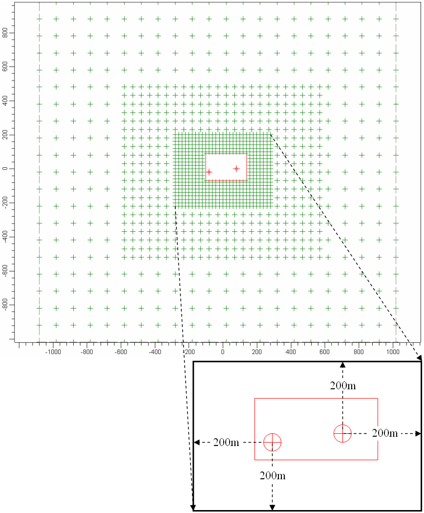
Subsection 14 (2) requires that receptors shall also be placed along the entire property boundary, and shall be separated by intervals of 10 metres or less. Receptors within the boundary shown in Figure 7.4 may be eliminated.
As set out in subsection 14 (5) of the Regulation, discrete receptors are required at locations where there are elevated points of impact such as apartment buildings and air intakes on nearby buildings. These are needed to ensure that maximum impacts are obtained. Other discrete receptors may be required for the types of receptors listed in subsection 30 (8) of the Regulation.
The above are minimal requirements to aid the modeller in defining adequate receptor coverage. The final extent and details are the responsibility of the modeller who must demonstrate that the point of impingement where concentration of the contaminant is highest has been identified. Certain stack characteristics, such as tall stacks, may inherently require larger receptor coverage.
Footnotes
- footnote[18] Back to paragraph A modeller is required to use site-specific meteorological data for an Emission Summary and Dispersion Modelling report prepared under section 30 of the Regulation (Upper Risk Thresholds) or section 32 of the Regulation (Site-Specific standard requests) or as required when issues a notice under section 13(2) of the Regulation.
- footnote[19] Back to paragraph Facilities wishing to use on-site meteorological observations for the purposes of dispersion modelling under the Regulation must ensure that the station meets all requirements set out in the Operations Manual for Air Quality Monitoring in Ontario (as amended) in terms of siting, calibration, operation and maintenance.