Model input data + Geographical information inputs
4.0 Model Input Data
Emission rate estimates are a key input parameter for an approved dispersion modelling assessment. Section 10 of the Regulation relates to facility operating conditions. Section 11 sets out the requirements for emission rates. Section 12 sets out the requirements to either “refine” emission estimates or mitigate air pollution when the combined effect of sections 10 and 11 indicate exceedences of air standards (or ministry POI Limits). The ESDM Procedure Document provides guidance on estimating emission rates to ensure that assessments of maximum point of impingement concentration are as accurate as possible and do not under-estimate actual concentrations.
Chapters 4 through 7 of the ADMGO document provide guidance on the model input parameter requirements within sections 13 through 17 of the Regulation.
4.1 Comparison of Screening and Other Approved Dispersion Model Requirements
Screening-level modelling assessments require the least amount of effort but should produce the most conservative results in most cases. The SCREEN3 approved dispersion model has straightforward input requirements and is further described in Chapter 4.1.1.
Conversely, air dispersion modelling assessments using a more advanced approved dispersion model such as the US EPA AERMOD model are somewhat more intensive than screening-level modelling. The modelling approach can be broken down into a series of steps. These are described in Chapters 4.1.2 AERMOD Air Dispersion Modelling.
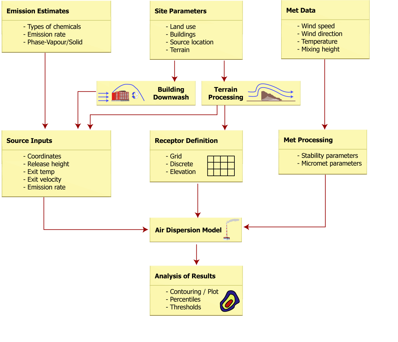
A general overview of the process typically followed for performing an air dispersion modelling assessment is presented in Figure 4.1. The figure is not meant to be exhaustive in all data elements, but rather provides a picture of the major steps involved in an assessment.
Figure 4.1: Generalized Process Flow Diagram for Performing an Air Dispersion Modelling Assessment
4.1.1 SCREEN3 Air Dispersion Modelling
The SCREEN3 model(13) was developed to provide an easy-to-use method of obtaining contaminant concentration estimates. To perform a modelling study using SCREEN3, data for the following input requirements shall be supplied:
- Source Type (Point, Flare, Area or Volume)
- Physical Source and Emissions Characteristics. For example, a point source requires:
- Emission Rate
- Stack Height
- Stack Inside Diameter
- Stack Gas Exit Velocity
- Stack Gas Exit Temperature
- Ambient Air Temperature
- Receptor Height Above Ground
- Meteorology: Although no data input is required, SCREEN3 provides users with the option to consider all wind speeds and stability classes, or a specific stability class and wind speed can be provided. Users should generally use all the wind speeds and stability class option.
- Building Downwash: If this option is used then building dimensions (height, length and width) must be specified. Downwash should always be selected for point sources located on or near buildings.
- Note: To ensure that potential downwash effects for stack heights that equal or exceed the Good Engineering Practice (GEP) height are considered (as they now are in AERMOD), stack heights greater than 2.5× the building height should be conservatively entered into SCREEN3 as 2.4× times the building height (see Chapter 4.6.1 for more information on the GEP).
- Terrain: SCREEN3 supports flat, elevated and complex terrain. If elevated or complex terrain is used, distance and terrain heights must be provided.
- Fumigation: SCREEN3 supports shoreline fumigation. If used, distance to shoreline must be provided.
As can be seen above, the input requirements are minimal to perform a screening analysis using SCREEN3. This model is normally used as an initial screening tool to assess single sources of emissions. SCREEN3 can be applied to multi-source facilities by conservatively summing the maximum concentrations for the individual emissions sources. The models discussed in the following sections have much more detailed options, allowing for greater characterization and more representative results.
4.1.2 AERMOD Air Dispersion Modelling
The more advanced approved dispersion models have many input options, and are described further throughout this document as well as in their own respective technical documents(1,5,6,13). An overview of the modelling approach and general steps for using models such as AERMOD are provided below. The general process for performing an air dispersion study using AERMOD includes:
- Process meteorological data using AERMET (unless using pre-processed data available from the ministry).
- Obtain digital terrain elevation data (if terrain is being considered – see section 16 of the Regulation).
- Incorporate building downwash using BPIP-PRIME (requires source and building information).
- Characterize the site – complete source and receptor information.
- Perform terrain data pre-processing (if required) for AERMOD dispersion model using AERMAP.
- Run “approved” version of the model.
footnote 14 - Visualize and analyze results.
It should be noted that AERMOD contains several output data processing algorithms that are specifically applicable to compliance with US EPA data processing requirements. For example, when the contaminant IDs for SO2, NO2 and PM2.5 are specified in the model inputs, the National Ambient Air Quality Standards (NAAQS) processing methodology is employed by default for these contaminants unless it is specifically disabled by the user. This will lead to erroneous predictions of maximum POI concentrations since the NAAQS metric is typically based on a multi-year average of ranked maximum daily values (i.e. for SO2 the 99th percentile of the maximum daily 1-hr values, averaged over 3 years would be calculated). Users should therefore either disable the output data processing options or specifically avoid choosing these default contaminant IDs within AERMOD (e.g. select “other”), since this would produce results that do not meet requirements of O. Reg. 419/05.
It should be noted, that paragraph 12 of subsection 26 (1) specifies that electronic copies of the input files that were used with the model and the output files that were generated by the model for each contaminant must be included in the ESDM report. This includes the output listing files (e.g. *.out, *.lst, which may differ if using a graphical interface program) in addition to any threshold violation files (e.g. *.max) and the contour plot files (e.g. *.plt) generated by the model.
The AERMOD modelling system is comprised of three primary components as outlined below and illustrated in Figure 4.2:
- AERMET – Meteorological Data Pre-processor
- AERMAP – Digital Terrain Data Pre-processor
- AERMOD – Air dispersion model
Figure 4.2: AERMOD Air Dispersion Modelling System
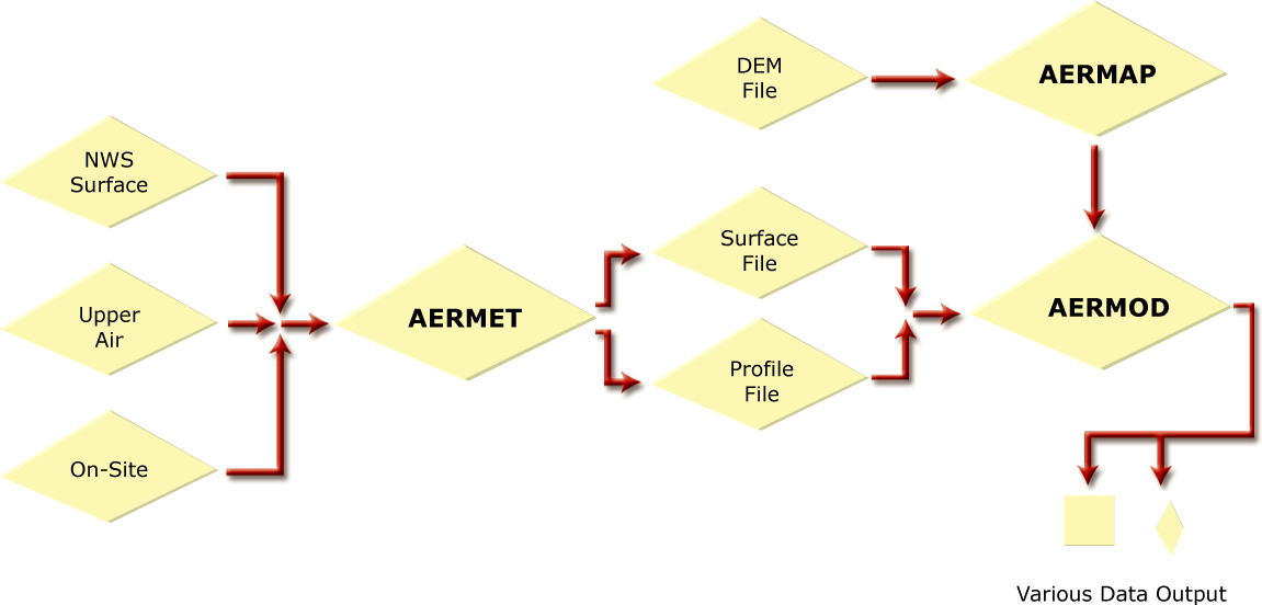
To successfully perform a complex terrain air dispersion modelling analysis using AERMOD, a modeller must complete the processing steps required by AERMET and AERMAP. See Chapter 6.3 for more information on meteorological data.
It should be noted that both the AERMET and AERMOD models are updated by the US EPA from time to time, and the ASHRAE model is periodically updated (historically every 4 years) by the American Society of Heating and Refrigeration and Air-Conditioning Engineers. There is a specific version of each of these models that is considered to be an “approved dispersion model”. In order for a specific version of these models to be considered to be an “approved dispersion model” version, the ministry will give notice that an updated version will be adopted. Such notice would typically be given via a posting on the Environmental Bill of Rights (EBR) Registry. Once such notice is given, the model versions specified in the notice will be law in Ontario until such time as a new notice is given to adopt another subsequent version.
AERMOD is a steady-state plume model. For the purpose of calculating 1-hour average concentrations, the plume is assumed to travel in a straight line without significant changes in stability as the plume travels from the source to a receptor. At distances on the order of tens of kilometres downwind, changes in stability, wind direction and wind speed are likely to cause this assumption to be invalid. For this reason, AERMOD shall not be used for modelling at receptors beyond 50 kilometres. AERMOD may also be inappropriate for some near-field modelling in cases where the wind field is very complex due to terrain or a nearby shoreline.
4.1.3 ASHRAE Air Dispersion Modelling
As an advanced model for same-structure contamination, ASHRAE has many input parameters, which are described briefly in this section with more detailed information in corresponding technical documents(
- Obtain building dimensions.
- Complete source and receptor information including:
- Emission Rate
- Stack height above main roof
- Stack inside diameter
- Stack gas exit velocity
- Distance from source to receptor/intake
- Is the stack capped or not?
- Wind speed range to be searched (for example, 2 – 12 m/s is a reasonable range over Ontario).
- Perform ASHRAE screening model run assuming a flush vent release.
- If results from the above screening model run failed to show compliance, perform calculations to obtain dimensions of building recirculation and wake zones; find the maximum roof top recirculation zone height between the source and the receptor.
- Perform advanced ASHRAE model run.
Note that:
- The above steps have to be carried out for each source-receptor combination.
- When defining the largest roof top recirculation zone height, all roof top recirculation zones caused by obstacles between the source and receptor in that specific source-receptor combination have to be included.
- When performing flush vent screening calculations, the stretched string distance should be used for the source to receptor distance (x). For all other cases, the downwind horizontal distance from the centre of the stack should be used.
- In complicated cases, projected building dimensions may have to be used.
- If using a version of ASHRAE that incorporates the surface roughness parameter, in order to prevent inconsistencies the roughness height used must be consistent with those used in other air dispersion modelling meteorological data files (e.g. AERMET).
Modellers are encouraged to contact the ministry’s Environmental Monitoring and Reporting Branch (EMRB) for specific guidance in more complex cases.
Information to be provided to the ministry with an assessment of self-contamination using ASHRAE should include a site drawing that shows plan and/or elevation views of the building with the building height, length and width, in addition to source and receptor (intake) locations and distances. Source details and parameters such as the stack height, flow rate and diameter should also be provided. Full calculations (including the wind speed ranges searched and the calculation of any intermediate parameters) must be provided in an Appendix, or electronically via an Excel spreadsheet.
4.2 “Regulatory Default” and “Non-Default” Option Use
The AERMOD model contains several options, which are set by default, that have been identified by the US EPA as “regulatory defaults”
- No stack-tip downwash (NOSTD);
- Missing data processing routine (MSGPRO);
- Bypass the calms processing routine (NOCALM);
- Gradual plume rise (GRDRIS);
- No buoyancy-induced dispersion (NOBID);
- Fast Area or Fast All options (FASTAREA, FASTALL);
- By-pass date checking for non-sequential met data file (NOCHKD);
- Deposition (WET, DRY);
- Conversion of NOx to NO2 (three methods OLM, PVMRM and ARM);
- Flat terrain (FLAT);
- Plume Depletion (WETDPLT, DRYDPLT);
- Side vents and horizontal caps (BETA); and
- Adjust u* and low wind speed options (LOWWIND).
Modellers shall use all default regulatory options in performing their modelling assessments. Also note that the US NAAQS processing methodology for SO2, NO2 and PM2.5 must be disabled if AERMOD is run using these contaminant names in the model input file.
Certain non-regulatory options may be used in a Tier 2 or Tier 3 assessment, but only for side vents and horizontal caps (see Chapter 4.5.3 Special Considerations for Horizontal Sources and Rain Caps), use of flat terrain and use of the FASTAREA/FASTALL options.
The ministry may consider whether it is appropriate to use deposition and plume depletion for Tier 3 modelling assessments, such as those requested for approval under paragraph 3 of subsection 11 (1) of the Regulation for a combined analysis of modelled and monitoring results. Other non-regulatory options may also be considered in a Tier 3 assessment, subject to ministry approval under section 7(1) of the Regulation. In such circumstances, modellers shall provide justification for, and obtain ministry (EMRB) approval for the use of non-regulatory options before submitting their modelling results to the ministry. Modellers are strongly encouraged to consult with the ministry in advance of conducting their model runs.
4.3 Coordinate System
Any modelling assessment will require a coordinate system be defined in order to assess the relative distances from sources and receptors and, where necessary, to consider other geographical features. Employing a standard coordinate system for all projects increases the efficiency of the review process while providing real-world information of the site location. AERMOD’s terrain pre-processor, AERMAP, requires digital terrain in Universal Transverse Mercator (UTM) coordinates. The UTM coordinate system uses metres as is its basic unit of measurement and allows for more precise definition of specific locations than latitude/longitude.
For more information on coordinate systems and geographical information inputs, see Chapter 5.0.
4.4 Averaging Periods (Conversion Factor)
Ministry POI Limits are expressed over certain averaging periods. As specified in section 17 of the Regulation, where a dispersion model is designed to determine a concentration for the specified averaging period, it shall be used as it was designed.
When a dispersion model is used that can only calculate concentrations for either a single averaging period or a limited range of averaging periods, conversion factors can be applied to estimate likely maximum concentrations over other averaging periods. The conversion allows model results from screening level assessments to be compared against ministry POI limits with their respective averaging periods. Models such as AERMOD provide the capability of providing 1, 2, 3, 4, 6, 8, 12, and 24-hour averages, as well as monthly and annual averages, therefore eliminating the need for conversion factors within these averaging periods. Conversion factors, however, are still required when modelling for averaging periods less than one hour. For example, for contaminants where the ministry POI Limit is based on a 30-minute averaging period, only the one-hour averaging period results obtained from the model can be converted to a 30-minute averaging period (see paragraph 3 of subsection 17 (1) of the Regulation).
Section 17 of the Regulation specifies averaging periods to be used, as well as when and how concentration conversions among averaging periods can occur, as follows:
Averaging periods
“17. (1) If a provision of this Part refers to an approved dispersion model being used in connection with a standard that applies to a specified averaging period, the following rules apply for the purposes of this Part:
- If an approved dispersion model was designed to be used for the specified averaging period, it shall be used as it was designed for that averaging period.
- If an approved dispersion model was not designed to be used for the specified averaging period but was designed to be used for an averaging period shorter than the specified averaging period, the model may be used as it was designed for the shorter averaging period if the result produced by the model is adjusted in accordance with subsection (2).
- If the specified averaging period is less than one hour and an approved dispersion model was designed to be used for a one hour period, the model may be used as it was designed for a one hour period if the result produced by the model is adjusted in accordance with subsection (2).
- If the use of an approved dispersion model is not authorized or required by paragraph 1, 2 or 3, the model shall not be used.
(2) If a provision of this Part refers to an approved dispersion model being used in connection with a standard that applies to a specified averaging period,
- the result produced by the approved dispersion model shall be multiplied by the amount determined in accordance with subsection (3), if the model is used under paragraph 2 of subsection (1); and
- the result produced by the approved dispersion model shall be divided by the amount determined in accordance with subsection (3), if the model is used under paragraph 3 of subsection (1).
(3) The amount referred to in clauses (2) (a) and (b) is the amount determined in accordance with the following formula:
(t0 ÷ t1)n
where,
- t0
- the shorter of,
- the averaging period that the approved dispersion model was designed to be used for, expressed in hours, and
- the specified averaging period, expressed in hours,
- t1
- the longer of,
- the averaging period that the approved dispersion model was designed to be used for, expressed in hours, and
- the specified averaging period, expressed in hours,
- n
- 0.28 or, if the Director is satisfied that another number would result in an adjustment that produces a more accurate prediction of the concentration of the relevant contaminant, the other number.
(4) If an approved dispersion model is used with respect to a person and contaminant to whom section 20 applies and Schedule 3 sets out more than one standard for the contaminant, using different averaging periods, the model shall be used with respect to each averaging period.
(5)This section does not apply if,
- The approved dispersion model that is used is the ASHRAE method of calculation and the model is being used in connection with a standard set out in Schedule 3 that applies to a 10 minute averaging period; or
- The approved dispersion model that is used is the method of calculation required by the Appendix to Regulation 346.
A range of averaging period conversion factors have been used in various studies, which are typically a function of the atmospheric stability. The equation given below is consistent with subsections 17 (2) and 17 (3) of the Regulation, and requires modellers to use a value for the exponent n that is based on neutral stability. However, the regulation allows the use of alternate stability dependant values of the exponent n
Equation 1:
C0 = C1 × F
where,
- C0
- the concentration at the averaging period t0
- C1
- the concentration at the averaging period t1
- F
- factor to convert from the averaging period t1 to the averaging period t0
= (t1 ⁄ t0)nand where,
- n
- 0.28
The formula could be used to calculate shorter averaging period concentrations such as a 10-minute ministry POI Limit starting from a modelled 1-hour average concentration. The equations can also be used to estimate a likely maximum 24-hour average concentration from a model that only produces 1-hour results. For example, output from SCREEN3 could be converted as follows:
C24hr = C 1hr × (1 hr ⁄ 24 hr)n
where:
- C 1hr and C 24hr
- are the maximum average concentrations respectively.
The following table (Table 4-1) lists some of the conversions that may be required by modellers to compare modelled results to ministry POI Limits.
| Convert From: | Convert To: | Multiply by: |
|---|---|---|
| 1hr | 10 min | 1.65 |
| 1hr | ½ hr | 1.2 |
| 1hr | 24hr | 0.4 |
| 1hr | Annual | 0.08 |
4.5 Defining Source Types
4.5.1 Selection, Description and Parameters
SCREEN3 and AERMOD support a variety of source types that can be used to characterize most emissions within a study area. Primary source types and their input requirements for both screening and the more advanced models are discussed below. Detailed descriptions on the input fields for these models can be found in the corresponding US EPA model User’s Guides, which are referenced in Chapter 10, and are for SCREEN3(13) and AERMOD(1).
Point Sources
Point sources are typically used to model releases from sources like stacks and isolated vents. Input requirements for point sources include:
SCREEN3
- Emission Rate: The emission rate of the contaminant.
- Stack Height: The stack height above ground.
- Stack Inside Diameter: The inner diameter of the stack.
- Stack Gas Exit Velocity [m/s] or Stack Gas Exit Flow Rate [m3/s]: Either the stack gas exit velocity or the stack gas exit flow rate must be given. The exit velocity can be determined from the following formula:
VS = 4Q ⁄ πdS2
Where:
- VS
- Exit Velocity (m/s)
- Q
- Flow Rate (m3/s)
- dS
- Stack Inside Diameter (m)
- Stack Gas Temperature: The temperature of the released gas in degrees Kelvin (K).
- Ambient Air Temperature: The average atmospheric temperature (K) in the vicinity of the source. If no ambient temperature data are available, assume a default value of 293 degrees K. For non-buoyant releases, the user shall input the same value for the stack temperature and ambient temperature.
- Receptor Height above Ground: This shall be used to model impacts at “flagpole” receptors. A flagpole receptor is defined as any receptor located above ground level, e.g., to represent the roof or balcony of a building. The default value is assumed to be 0.0 m (i.e., ground-level receptors).
- Urban/Rural Option: Specify either Urban or Rural conditions to use the appropriate dispersion coefficient. Chapter 5.4.5 Defining Urban and Rural Conditions provides guidance on determining rural or urban conditions.
AERMOD
- Source ID: An identification name for the source being defined, up to 8 characters in length.
- X Coordinate: The x (east-west) coordinate for the source location in metres (centre of the point source).
- Y Coordinate: Enter here the y (north-south) coordinate for the source location in metres (centre of the point source).
- Base Elevation: The elevation of the base of the source. The model only uses the source base elevation if Elevated terrain is being used.
- Release Height above Ground: The source release height above the ground in metres.
- Emission Rate: The emission rate of the contaminant in grams per second.
- Stack Gas Exit Temperature: The temperature of the released gas in degrees Kelvin.
- Stack Gas Exit Velocity: The stack gas exit velocity in metres per second or the stack gas flow rate (see above Chapter on SCREEN3).
- Stack Inside Diameter: The inner diameter of the stack.
Area Sources
Area sources are used to model low level or ground level releases where releases occur from a two-dimensional flat plane with no temperature, velocity or initial mixing or dilution (e.g., landfills, storage piles, slag dumps, lagoons). SCREEN3 allows definition of a rectangular area while AERMOD accepts rectangular areas that may also have a rotation angle specified relative to a north-south orientation. AERMOD can also handle circular and polygon shaped area sources.
SCREEN3
- Emission Rate: The emission rate of the contaminant. The emission rate for area sources is entered as an emission rate per unit area (g/(s-m2)).
- Source Release Height: The source release height above ground.
- Larger Side Length of Rectangular Area: The larger side of the rectangular source in metres.
- Smaller Side Length of Rectangular Area: The smaller side of the rectangular source in metres.
- Receptor Height above Ground [m]: This shall be used to model impacts at “flagpole” receptors. A flagpole receptor is defined as any receptor that is located above ground level, e.g., to represent the roof or balcony of a building. The default value is assumed to be 0.0 m (i.e., ground-level receptors).
- Wind Direction Search Option: Since the concentration at a particular distance downwind from a rectangular area is dependent on the orientation of the area relative to the wind direction, the SCREEN model provides the user with two options for treating wind direction. The modeller shall use the regulatory default option (“yes”) which results in a search of a range of wind directions. See US EPA SCREEN3 Model User’s Guide(13) for more detailed information.
AERMOD
- Source ID: An identification name for the source being defined, up to 8 characters in length.
- X Coordinate: The x (east-west) coordinate for the vertex (corner) of the area source that occurs in the southwest quadrant of the source. Units are in metres.
- Y Coordinate: The y (north-south) coordinate for the vertex (corner) of the area source that occurs in the southwest quadrant of the source. Units are in metres.
- Base Elevation: The elevation of the base of the source. The model only uses the source base elevation if elevated terrain is being used. The default unit is metres.
- Release Height above Ground [m]: The release height above ground in metres.
- Emission Rate [g/(s-m2)]: Enter the emission rate of the contaminant. The emission rate for area sources is entered as an emission rate per unit area. The same emission rate is used for both concentration and deposition calculations.
- Options for Defining Area: AERMOD can have rectangular, circular or polygon areas defined (see US EPA(1) for details).
Note: Receptors may be placed within the area and at the edge of an area. AERMOD will integrate over the portion of the area that is upwind of the receptor. The numerical integration is not performed for portions of the area that are closer than 1 metre upwind of the receptor. Therefore, caution should be used when placing receptors within or adjacent to areas that are less than a few metres wide. In such cases, modellers are encouraged to contact ministry (EMRB) to discuss receptor placement.
Volume Sources
Volume sources are used to model releases from a three-dimensional box that represents the evenly-mixed emissions of a contaminant from the source. A variety of industrial sources can be represented by volume sources, including building roof monitors, fugitive leaks from an industrial facility, multiple vents, and stacker drop points.
SCREEN3
- Emission Rate: The emission rate of the contaminant in grams per second (g/s).
- Source Release Height: The source release height above ground surface. This is typically the centre of the volume source.
- Initial Lateral Dimension: See Table 4-2 for guidance on determining initial dimensions. Units are metres.
- Initial Vertical Dimension: See Table 4-3 for guidance on determining initial dimensions. Units are metres.
- Receptor Height above Ground [m]: This shall be used to model impacts at “flagpole” receptors. A flagpole receptor is defined as any receptor which is located above ground level, e.g., to represent the roof or balcony of a building. The default value is assumed to be 0.0 m (i.e., ground-level receptors).
| Type of Source | Procedure for Obtaining Initial Dimension |
|---|---|
| Single Volume Source | SYo = side length ⁄ 4.3 |
| Line Source Represented by Adjacent Volume Sources | SYo = side length ⁄ 2.15 |
| Line Source Represented by Separated Volume Sources | SYo = centre to centre distance ⁄ 2.15 |
Source: US EPA, 1995 User’s Guide for the Industrial Source Complex (ISCST3) Dispersion Models - Volume I, EPA-454/B-95-003a. US EPA. Research Triangle Park, NC 27711.
| Type of Source | Procedure for Obtaining Initial Dimension |
|---|---|
| Surface-Based Source (he ~ 0) | SZo = vertical source dimension ⁄ 2.15 |
| Elevated Source (he > 0) on or Adjacent to a Building |
SZo = building height ⁄ 2.15 |
| Elevated Source (he > 0) not on or Adjacent to a Building |
SZo = vertical source dimension ⁄ 4.3 |
Source: US EPA, 1995 User’s Guide for the Industrial Source Complex (ISCST3) Dispersion Models - Volume I, EPA-454/B-95-003a. US EPA. Research Triangle Park, NC 27711.
AERMOD
- Source ID: An identification name for the source being defined, up to 8 characters in length.
- X Coordinate: The x (east-west) coordinate for the source location in metres. This location is the centre of the volume source.
- Y Coordinate: The y (north-south) coordinate for the source location in metres. This location is the centre of the volume source.
- Base Elevation: The elevation of the base of the source. The model only uses the source base elevation if elevated terrain is being used. The default unit is metres.
- Release Height above Ground: The release height above ground surface in metres (centre of volume).
- Emission Rate [g/s]: The emission rate of the contaminant in grams per second. The same emission rate is used for both concentration and deposition calculations.
- Length of Side: The length of the side of the volume source in metres. The volume source cannot be rotated and has the X side equal to the Y side (square).
- Building Height (If On or Adjacent to a Building): If the volume source is elevated and is on or adjacent to a building, then the modeller needs to specify the building height. The building height can be used to calculate the Initial Vertical Dimension of the source. Note that if the source is surface-based, then this is not applicable.
- Initial Lateral Dimension [m]: This parameter is calculated by choosing the appropriate condition in Table 4-2. This table provides guidance on determining initial dimensions. Units are in metres.
- Initial Vertical Dimension [m]: This parameter is calculated by choosing the appropriate condition in Table 4-3. This table provides guidance on determining initial dimensions. Units are in metres.
Line Sources
Examples of line sources are conveyor belts and rail lines. SCREEN3 does not have a default line source type, whereas AERMOD does. There are a number of different approaches that can be used to simulate line sources. These generally include use of a series of area or volume sources to define a line source (e.g. a roadway source), in addition to the release height of the emissions and the initial plume spread. The sources can either be located adjacent to one another, or separated by a specified distance. The AERMOD line source is based on the area source approach, and uses a single area source to represent straight line segments. Additionally, some commercially available software products have built-in a “line sources” generating function for AERMOD, which use either the separated or adjacent volume source approach, or the adjacent area source approach. For additional guidance on modelling roadway type line sources, see Chapter 4.5.3.
Open Flare Sources
Flares are used as control devices for a variety of sources. Enclosed flares are typically modelled as normal point sources when using SCREEN3 or AERMOD. Open flares however, are quite different from traditional “stack type” point sources because they have unique exhaust characteristics. Open flares produce extremely hot (and therefore buoyant) and turbulent exhaust streams. Also, open flares typically have a jet-like flame, and exhaust/combustion contaminants are emitted from a plume that starts at the top of the flame, or the flame tip. Due to these unique characteristics, open flares must be modelled differently than typical stack type point sources. For more information, please refer to the “Technical Bulletin: Modelling Open Flares under O. Reg. 419/05”, dated July 2016.
In general, they are modelled as point sources with modified exhaust parameters. SCREEN3 supports modelling open flares directly through its flare source type, as this model modifies the exhaust parameters automatically. The AERMOD model does not automatically modify the exhaust parameters, and as such they must be calculated by the user before being input into the model.
SCREEN3
When modelling emissions from flares using the SCREEN3 model, only the flare source type should be employed, with the required input parameters as outlined below.
- Emission Rate: The emission rate of the contaminant in grams per second (g/s).
- Flare Stack Height: The stack height above ground (m).
- Total Heat Release Rate: The heat release rate in calories per second (cal/s) for the flare.
- Receptor Height above Ground: This shall be used to model impacts at “flagpole” receptors. A flagpole receptor is defined as any receptor which is located above ground level, e.g., to represent the roof or balcony of a building. The default value is assumed to be 0.0 m (i.e., ground-level receptors).
Note 1: US EPA's SCREEN3 model calculates plume rise for flares based on an effective buoyancy flux parameter. An ambient temperature of 293 K is assumed in this calculation and therefore no ambient temperature is entered by the user. It is assumed that 55% of the total heat is lost due to radiation. Plume rise is calculated from the top of the flame, assuming that the flame is bent 45 degrees from the vertical. SCREEN3 calculates and prints out the effective release height for the flare.
Note 2: For Flare releases, EPA’s SCREEN3 model assumes a stack gas exit velocity (Vs) of 20 m/s, an effective stack gas exit temperature (Ts) of 1,273 K, and calculates an effective stack diameter based on the heat release rate.
AERMOD
AERMOD does not have a specific source type option for open flare sources. Instead, flare emissions are modelled as point sources, with the modified exhaust parameters. These parameters need to be modified to consider buoyancy flux reductions associated with radiative heat losses, in addition to inclusion of the flame length in estimating the effective release height(16,17). The effective parameters are as follows:
- Modified or “effective” stack height (Hsl)
- Effective exit velocity (Veff)
- Effective stack diameter (Deff)
These are known as flare “pseudo-parameters” because they are calculated in a manner to simulate the behaviour of the exhaust plume as if it were a stack type point source, emitted from a height equal to the tip of the flame. The remaining parameters (effective diameter and effective exit velocity) are also calculated at the flame tip, considering the expected expansion and air entrainment into the plume, while conserving buoyancy and momentum flux(18). The ministry has revised the methodology to be used when modelling open flares in Ontario, and developed the Technical Bulletin: Modelling Open Flares under O. Reg. 419/05, July 2016 to provide specific guidance for modelling these sources. The Technical Bulletin provides background information, the revised methodology and a stepwise procedure for the calculation of the required flare pseudo-parameters. When the AERMOD model or other approved dispersion models are used to model open flare sources, the approach and equations outlined in the Technical Bulletin are to be used to characterize the source parameters. Please refer to the Technical Bulletin for these details when modelling open flares.
Note that all data, assumptions and calculations for the flare pseudo-parameters must be included as part of the supporting documentation for the assessment.
4.5.2 Combining Individual Sources into Volume, Area and Single Point Sources
There are cases where a facility could have a number of release points from vents and short stacks in a confined area at the facility. To simplify the modelling when there are many release points, a modeller may conservatively combine these stacks/vents into a volume source, an area source or a single point source.
The following factors shall be considered when selecting potential sources for combination into a single source:
- source characteristics (e.g. exit velocity, temperature, stack/source height) of the individual stacks or vents must be similar,
- emission rates from the individual release points must be similar (i.e. there are no sources with significantly larger emission rates),
- sources must be located in the same general vicinity, and
- the property line must not be too far from the group of stacks/vents.
When employing this approach, the choices of size and location of volume or area sources or the stack parameters for a single stack representing a group must be selected conservatively. For example:
- for combining multiple stacks into a single stack, the parameters for the single stack shall not result in a larger plume rise than would have occurred for the large majority of the stacks being combined (i.e. the exit velocity selected should be conservative), and
- for combining multiple sources into a single volume source, the size of a volume source selected to represent the group of sources shall only consider the volume on which the sources are located and from which the emissions would be released. In most cases, the volume source height would be same as the building/structure height or lower.
Modellers are encouraged to contact EMRB for specific guidance in these situations.
Output of Results for Groups of Sources
When modelling is performed for a number of individual stacks, volume sources or area sources, the use of source groups enable modelling results to be output for specific combinations of sources. The default in AERMOD is the creation of source group “all” that considers all the sources at the same time. Analysis of specific groups of sources, such as process vents, site roadways, combustion equipment, etc. can be performed by using the SRCGROUP option. Conversely, individual sources may be assigned to a separate group to determine the concentrations generated by each individual source. It should be noted however that when this is done for individual sources or groups the results reflect the maximum predicted concentrations from each of these, rather than the contribution to the overall maximum from all sources combined.
4.5.3 Special Considerations
During some air quality studies, certain source configurations or source types may be encountered that require special attention. Some examples include horizontal sources or emissions from storage tanks. The following sections outline modelling techniques on how to account for the special characteristics of such scenarios.
Shoreline Fumigation
Shoreline fumigation is a phenomenon that may occur along the shore of an ocean or a large lake. When the land is warmer than the water, a breeze forms as the warmer, lighter inland air rises. As the stable, cooler air from over the water moves inland, it is heated from below, resulting in a turbulent boundary layer of air that rises with downwind distance from the shoreline. The plume from a tall stack source located near the shoreline may intersect this turbulent layer and be rapidly mixed to the ground, a process called “fumigation,” resulting in high ground level concentrations. AERMOD does not treat the effects of shoreline fumigation. In these and other situations, the use of specific models may be required by the ministry under section 7 of the Regulation.
Shoreline fumigation need only be assessed from tall stacks as it does not occur with respect to emissions from ground level sources modelled as area or volume sources. The SCREEN3 model includes an option to assess whether shoreline fumigation may occur as a result of stack emission sources located near a large lake or water body. Examples of larger lakes or water bodies that could lead to fumigation include the Great Lakes, Georgian Bay, Lake St. Clair, and others.
Generally, facilities located within approximately 1 km of the shoreline of a larger lake or water body, that emit contaminants from taller stack sources greater than 50 metres in height, need assess the potential for shoreline fumigation to occur using the SCREEN3 model. Should the screening assessment show that shoreline fumigation may occur, the use of an alternative model (e.g. CALPUFF, Shoreline Dispersion Model) may be required by a notice issued under section 7 of the Regulation.
Multiple Stacks
When the plumes from multiple closely-spaced stacks or flues merge, the plume rise can be enhanced. Briggs(19) has proposed equations to account for this. The reader is referred to that document for further details. Most models do not explicitly account for enhanced plume rise from this cause, and most regulatory agencies do not permit it to be considered in regulatory applications of modelling, with one exception. That exception is the case of a single stack with multiple flues, or multiple stacks located very close together (less than approximately one stack diameter apart). In these cases, the multiple plumes may be treated as a single plume. To do this, a pseudo stack diameter is used in the calculations, such that the total volume flow rate of the stack gases is correctly represented.
Horizontal Sources and Rain Caps
Both horizontal flues and vertical flues with rain caps have little or no initial vertical velocity. Plume rise calculations in most models (including AERMOD and SCREEN3) take into account both rise due to vertical momentum of the plume as it leaves the stack and the buoyancy of the plume. This may result in an over-prediction of the plume rise, and resulting under-prediction of ground-level concentrations, in these models.
This problem can be alleviated by modifying the source input parameters to minimize the effects of momentum while leaving the buoyant plume rise calculations unchanged. The US EPA outlines such an approach in its Model Clearinghouse Memo 93-II-09(20). The approach is also expressed, in part, in Tikvart(21). This approach is to reduce the stack gas exit velocity to 0.001 m/s, and calculate an equivalent diameter so that the buoyant plume rise is properly calculated. To do this, the stack diameter is specified to the model such that the volume flow rate of the gas remains correct.
In the case of horizontal flues, there will be no stack tip downwash (i.e. reduction of the plume height by an amount up to three times the stack diameter), so that option must be turned off. In the case of vertical flues with rain caps, there will be frequent occurrences of stack tip downwash. The effect of the stack tip downwash however may be underestimated in the model and thus must be corrected. This is done somewhat conservatively by turning off the stack tip downwash and lowering the specification of the stack height by three times the actual stack diameter (i.e. the maximum effect of stack tip downwash). However, the modified stack height must not be reduced to be below the roof level.
With the above references in mind, it should be noted that larger diameters associated with reduced exit velocities can cause issues with the PRIME algorithm. As a result, the ministry’s approach is to use an exit velocity of 0.1 m/s, or a velocity based on limiting the exit diameter to 5 times the actual diameter up to a maximum of 5 metres. This exit velocity still effectively eliminates momentum flux and can produce parameters that will not impede model execution.
The current AERMOD model includes a non-default beta option for modelling releases from capped and horizontal discharge stacks. EPA model developers found that the Model Clearinghouse procedure is not appropriate for sources subject to building downwash influences with the PRIME downwash algorithm. The use of an effective diameter adjusted to maintain flow rate could produce unrealistic results with the PRIME algorithm. In the AERMOD capped and horizontal releases options, the vertical momentum is suppressed while the buoyancy of the plume is conserved without modifying the stack parameters.
The two source types are:
- POINTCAP for capped stacks, and
- POINTHOR for horizontal releases.
For each of these source types, the user must specify the actual stack parameters of release height (m), exit temperature (K), exit velocity (m/s), and stack diameter (m) using the SO SRCPARAM card as if the release were a non-capped vertical point source. The AERMOD model performs the necessary adjustments internally to account for plume rise and stack-tip downwash. For horizontal releases, the model assumes that the release is oriented with the wind direction. For PRIME-downwashed sources, the user-specified exit velocity for horizontal releases is treated initially as horizontal momentum in the downwind direction.
The capped and horizontal beta option in AERMOD produces results that are very similar to those using the previously described ministry approach. The beta options for capped and horizontal releases should be used when modelling with AERMOD. When modelling with SCREEN3, the following step-by-step approach should be used. In this discussion,
- V
- actual stack gas exit velocity
- V’
- stack gas exit velocity as entered into the model
- D
- actual stack inside diameter
- D’
- stack inside diameter as input to the model
- H
- actual stack height
- H’
- stack height input to the model
For the source of consideration, modify its parameters as follows:
- Set V’ = 0.1 m/s or a velocity based on limiting the exit diameter to 5 times the actual diameter up to a maximum of 5 metres
- Set D’ = D × SQRT (V ⁄ V’)
- If the source is a vertical stack with a rain cap, account for the frequent stack tip downwash by reducing the stack height input to the model by three times the actual stack diameter: H’ = H − 3D
Roadways
Modelling emissions from roadways and haul roads can be challenging. Historically, none of the advanced dispersion models contained a specific line or roadway source type that could be best used to simulate dispersion of emissions from the surface of a roadway. Instead, roadway sources are typically simulated using a series of volume or area sources. A new line source type was recently added to the AERMOD model, which is based on the area source approach, and uses a single area source for each straight line segment. These types of sources however, do not appropriately simulate the turbulence and added dispersion that occurs in the wake of moving vehicles. Because of this phenomenon, roadway modelling results produced by AERMOD can be overly conservative in some circumstances. This is particularly true of predicted concentrations at receptors located in the area of the perpendicular intersection of road sources and the property boundary. This is likely due to model limitations for receptors at close distances to sources with low release heights and the lack of plume rise.
In order to address these issues, the ministry recommends the following:
- Roadways may be simulated using a series of adjacent or separated volume or area sources. The ministry would prefer that the volume source approach be employed.
- Model receptors should not be placed directly on the roadways, including points where the property line intersects the roadway.
- Model receptors along a property line that intersects a roadway can be offset from the roadway edge by a distance of 1.5 × the road width
The US EPA has also faced similar challenges related to modelling emissions and impacts of haul roads. In 2009 the US EPA formed the Haul Road Workgroup which was comprised of air dispersion modellers from federal, state and local regulatory agencies. The group focussed on challenges related to air dispersion modelling aspects rather than those related to emissions estimation. In particular, the group studied different modelling options and approaches using AERMOD, and produced a memorandum in 2012 that included some specific recommendations regarding the modelling approach(22). The ministry suggests that the recommendations in this memorandum be followed in modelling emissions from haul roads in Ontario.
In certain circumstances, a notice under section 7 of the Regulation may be issued to allow use of a traffic air dispersion model such as CAL3QHCR or CALINE4 instead of the approach described above. Further details on these models can be found in Appendix A: Alternative Models.
Pits and Quarries
Emissions from pits and quarries behave differently than ground level sources. Research indicates that a portion of the emissions are retained in the pit, and that they are generally emitted from a smaller area of the pit opening. AERMOD contains an OPENPIT source type that simulates the unique manner in which emissions are emitted from pits and quarries.
Some of the key parameters required by the OPENPIT source are as follows:
- Source Location: This is the x and y coordinates of the southwest corner of the source, in metres.
- Base Elevation: The elevation of the pit opening (i.e. the top of the pit, which is where the emissions are simulated to occur). The model only uses this if terrain data is being used. The default unit is metres.
- Release Height: This is the average release height above the base of the pit in metres (centre of volume). This parameter cannot exceed the effective depth of the pit, which is calculated based on the volume of the pit and specified length and width. Where there are multiple sources within the pit, the specified release height should be based on the average source heights within the pit.
- Length of Sides: The length and width of the pit opening in metres. The model uses these values to calculate the effective depth of the pit.
- Pit Volume: The total volume of the pit in cubic metres. The model uses this value to calculate the effective depth of the pit.
It should be noted that when using the OPENPIT source type in AERMOD, the model simulates the release of emissions at the top of the pit, from an “effective” area source. As such, modifying the terrain or source base elevation of the pit should only be done based on project development information to account for modifications such as initial topsoil removal. In cases where the elevations in the DEM files reflect an existing pit, use of the existing base elevation (i.e. the pit floor) as the source base elevation in the model will incorrectly result in the model assigning this elevation to the top of the pit (i.e. the top of the pit will be incorrectly placed at the pit floor). It may be more appropriate to model these sources using different approaches, such as volume or area sources, depending on the situation. Modellers should contact EMRB for further guidance, as necessary.
Liquid Storage Tanks
Storage tanks are generally of two types—fixed roof tanks and floating roof tanks. In the case of fixed roof tanks, most of the contaminant emissions occur from a vent, with some additional contribution from hatches and other fittings. In the case of floating roof tanks, most of the contaminant emissions occur through the seals between the roof and the wall and between the deck and the wall, with some additional emissions from fittings such as ports and hatches.
Approaches for modelling impacts of emissions from various types of storage tanks are described below.
Fixed roof tanks:
Model fixed roof tanks as a point source representing the vent, which is usually in the centre of the tank, and representing the tank itself as a building for downwash calculations.
Floating roof tanks:
Model floating roof tanks as a circle of eight (or more) point sources, representing the tank itself as a building for downwash calculations. Distribute the total emissions equally among the circle of point sources.
All tanks:
There is virtually no plume rise from tanks. Therefore, the stack parameters for the stack gas exit velocity and stack diameter shall be set to near zero for the stacks representing the emissions. In addition, stack temperature shall be set equal to the ambient temperature. This is done in AERMOD by entering a value of 0.0 for the stack gas temperature.
Note that it is very important to either turn off stack tip downwash or to set the diameter to near zero. With low exit velocities and larger diameters, stack tip downwash will be calculated. Since all downwash effects are being calculated as building downwash, the additional stack tip downwash calculations would be inappropriate. Since the maximum stack tip downwash effect is to lower plume height by three stack diameters, a very small stack diameter effectively eliminates the stack tip downwash. Table 4-4 presents values of stack parameters used in modelling tanks.
| Velocity | Diameter | Temperature |
|---|---|---|
| Near zero i.e.0.001 m/s |
Near zero i.e.0.001 m |
Ambient – 0.0 sets models to use ambient temperature |
4.5.4 Variable Emissions
The AERMOD model supports variable emission rates. This allows for modelling of source emissions that may fluctuate over time. Emission variations can be characterized across many different periods including hourly, daily, monthly and seasonally. For more information on emission estimating, please refer to the ESDM Procedure Document.
Wind Erosion
Modelling of emissions from sources susceptible to wind erosion, such as storage piles, shall be accomplished using variable emissions.
The AERMOD model allows for emission rates to be varied by wind speed. This allows for more representative emissions from sources that are susceptible to wind erosion, particularly waste piles that can contribute to particulate emissions. Once a correlation between emissions and wind speed categories is established, the models will then vary the emissions based on the wind conditions in the meteorological data.
Non-Continuous Emissions
Sources of emissions at some locations may emit only during certain periods of time. Emissions can be varied within the AERMOD model by applying factors to different time periods.
For example, for a source that is non-continuous, a factor of 0 is entered for the periods when the source is not operating or inactive. A factor of 0.5 decreases the mass emission rate for the selected time periods to 50%. Note that only the mass emission rate is affected with the use of these factors. The other source parameters such temperature and exit velocity remain constant. Start-ups and shutdowns are examples of non-continuous emissions which could use the variable emission rate options. Model inputs for variable emissions rates can include the following time periods:
- Hour-of-day;
- Monthly;
- Seasonally;
- Wind speed;
- By Season and hour-of-day; and
- By Season, hour-of-day, and day-of-week.
An external hourly input file can be prepared in which all parameters of specified sources including mass emission rate, exit velocity and temperature may be varied on an hour-by-hour basis over the entire modelling period.
4.6 Building Impacts
Buildings and other structures near a relatively short stack can have a substantial effect on plume transport and dispersion, and on the resulting ground-level concentrations that are observed. There has long been a generalized approach that a stack should be at least 2.5 times the height of adjacent buildings. Beyond that, much of what is known of the effects of buildings on plume transport and diffusion has been obtained from wind tunnel studies and field studies.
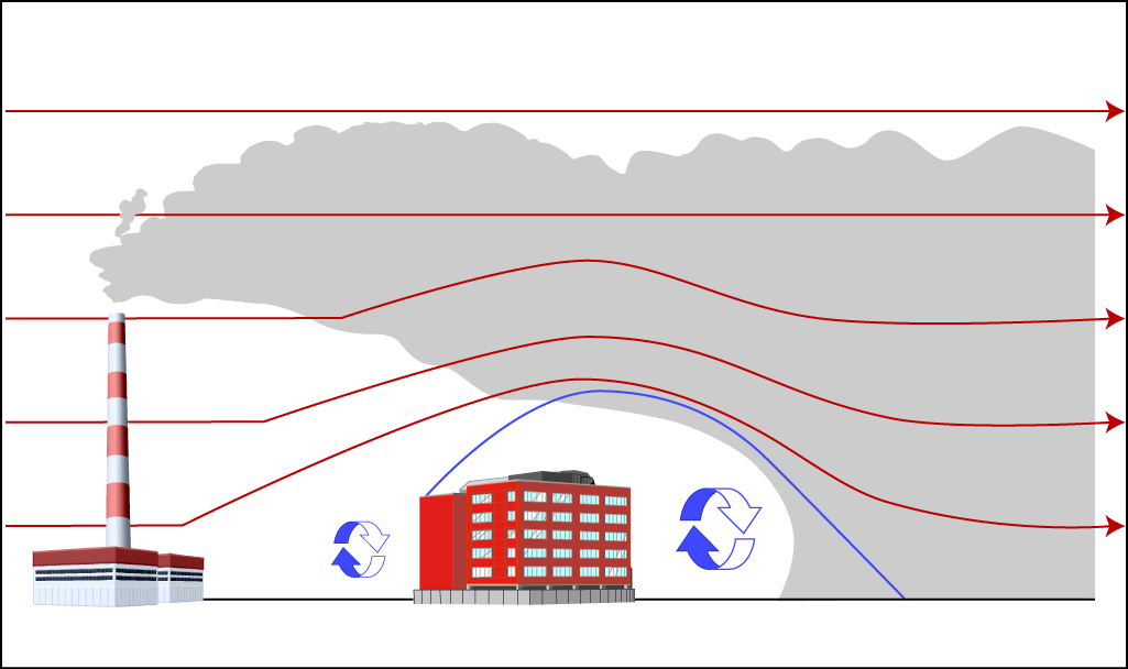
When the airflow meets a building (or other obstruction), it is forced up and over the building. On the lee side of the building, the flow separates, leaving a closed circulation zone containing lower wind speeds. Farther downwind, the air flows downward again. In addition, there is more shear and, as a result, more turbulence. This is the turbulent wake zone (see Figure 4.3).
If a plume gets caught in the cavity, very high concentrations can result. If the plume escapes the cavity, but remains in the turbulent wake, it may be carried downward and dispersed more rapidly by the turbulence. This can result in either higher or lower concentrations than would occur without the building, depending on whether the reduced height or increased turbulent diffusion has the greater effect.
The height to which the turbulent wake has a significant effect on the plume is generally considered to be about the building height plus 1.5 times the lesser of the building height or width. This results in a height of 2.5 times the building heights for cubic or squat buildings, and less for tall, slender buildings. Since it is considered good engineering practice to build stacks taller than adjacent buildings by this amount, this height came to be called “good engineering practice” (GEP) stack height. Figure 4.3 graphically presents the building downwash concept where the presence of buildings form localized turbulent zones that can readily draw contaminants down to ground level.
Figure 4.3: Building Downwash Effect
4.6.1 Stack Height for Certain New Sources of Contaminants: Good Engineering Practice (GEP) Stack Heights And Structure Influence Zones
GEP Stack Heights are the stack heights that the US EPA(26) requires to avoid having to consider building downwash effects in dispersion modelling assessments. The definition of GEP is stack heights equal to the building height plus 1.5 times the smaller of the building height or width.
Section 15 of the Regulation specifies the stack height to be used in modelling for new stacks as follows:
Stack height for certain new sources of contaminant
“15. (1) This section applies to a source of contaminant if all of thefollowing criteria are met:
- The source of contaminant dischargescontaminants directly into the natural environment.
- Construction of the source of contaminantbegan after November 30, 2005.
- No application was made on or before November 30, 2005 for a certificate of approval in respect of the source of contaminant.
- The source of contaminant is located in an area around a structure that is bounded by a circle that has a radius of five times the lesser of the following:
- The height above ground level of the structure.
- The greatest width presented to the wind by the structure, measured perpendicularly to the direction of the wind.
(2) If an approved dispersion model other than the ASHRAE method of calculation is used for the purposes of this Part with respect to a source of contaminant to which this section applies, the height at which contaminants are discharged into the air from the source of contaminant that is used with the model must be the lower of the following heights:
- The actual height above ground level at which contaminants are discharged into the air from the source of contaminant.
- The higher of the following heights:
- Sixty-five metres.
- The height described in subsection (3).
(3) The height referred to in sub paragraph 2 ii of subsection (2) is the height determined by the following formula:
A + (1.5 × B)
where,
- A
- the height above ground level of the structure referred to in paragraph 4 of subsection (1),
- B
- the lesser of,
- the height above ground level of the structure referred to in paragraph 4 of subsection (1), and
- the greatest width presented to the wind by the structure referred to in paragraph 4 of subsection (1), measured perpendicularly to the direction of the wind.
(4) If paragraph 4 of subsection (1) applies to a source of contaminant in respect of more than one structure, the references in subsection (3) to the structure referred to in paragraph 4 of subsection(1) shall be deemed to be references to the structure for which the height referred to in subparagraph 2 ii of subsection (2) is the greatest.
(5) This section applies only if the approved dispersion model is used with respect to a person and contaminant to which section 20 applies.”
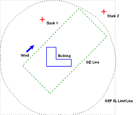
Building downwash shall be considered for point sources that are within the Area of Influence (see Figure 4.4) of a building. For US EPA regulatory applications, a building is considered sufficiently close to a stack to cause wake effects when the distance between the stack and the nearest part of the building is less than or equal to five (5) times the lesser of the building height or the projected width of the building.
Distancestack-bldg ≤ 5L
For point sources within the Area of Influence, building downwash information (direction-specific building heights and widths) shall be included in the modelling project. Using BPIP-PRIME, a modeller can compute the direction-specific building heights and widths.
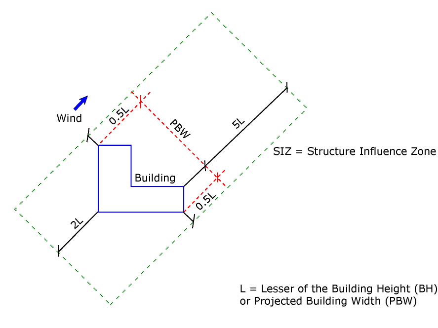
Structure Influence Zone (SIZ): For downwash analyses with direction-specific building dimensions, wake effects are assumed to occur if the stack is within a rectangle composed of two lines perpendicular to the wind direction, one at 5L downwind of the building and the other at 2L upwind of the building, and by two lines parallel to the wind direction, each at 0.5L away from each side of the building, as shown below. L is the lesser of the height or projected width. This rectangular area has been termed a SIZ. Any stack within the SIZ for any wind direction is potentially affected by GEP wake effects for some wind direction or range of wind directions, and shall be included in the modelling project. Figure 4.4 shows the SIZ around a building.
Figure 4.4: GEP 5L and Structure Influence Zone (SIZ) Areas of Influence (after US EPA(23))
When determining the potential building effects, the BPIP program searches through 360° of wind directions to determine the SIZ for each wind direction, and the point sources that will potentially be affected by downwash, for each wind direction. Figure 4.5 shows the potential SIZ around the entire building, and illustrates how different sources could be affected by downwash, depending on their location relative to the building.
Figure 4.5: GEP 360° 5L and Structure Influence Zone (SIZ) Areas of Influence (US EPA(27))
AERMOD versions prior to version 11059 used the GEP height as a limitation on plume downwash calculations, i.e., downwash was not calculated for stacks greater than the GEP height. This resulted in a discontinuity in model results for stacks that were slightly greater than the GEP height. AERMOD versions 11059 and later have been updated such that building downwash is calculated for all stacks in the influence zone/area, including those which are greater than the GEP height. Please note that the Regulation requires the use of the “approved” version of AERMOD, which is the most recent version that has been posted on the EBR.
4.6.2 Defining Buildings
All of the US EPA models allow for the consideration of building downwash. SCREEN3 considers the effects of a single building while AERMOD can consider the effects of complicated sites consisting of hundreds of buildings. This results in different approaches to defining buildings which are described below.
SCREEN3 Building Definition
Defining buildings in SCREEN3 is straightforward, as only one building requires definition. The following input data is needed to consider downwash in SCREEN3:
- Building Height: The physical height of the building structure in metres.
- Minimum Horizontal Building Dimension: The minimum horizontal building dimension in metres.
- Maximum Horizontal Building Dimension: The maximum horizontal building dimension in metres.
If using Automated Distances or Discrete Distances option, wake effects are included in any calculations made. Cavity calculations are made for two building orientations, first with the minimum horizontal building dimension along-wind, and second with the maximum horizontal dimension along-wind. The cavity calculations are summarized at the end of the distance-dependent calculations (see SCREEN3 User’s Guide(13) Chapter 3.6 for more details).
AERMOD Building Definition
The inclusion of the PRIME algorithm(24) to compute building downwash has generally produced more accurate results in air dispersion models. Unlike the earlier algorithms used in ISCST3, the PRIME algorithm:
- accounts for the location of the stack relative to the building;
- accounts for the deflection of streamlines up over the building and down the other side;
- accounts for the effects of the wind profile at the plume location for calculating plume rise;
- accounts for contaminants captured in the recirculation cavity to be transported to the far wake downwind (this was ignored in the earlier algorithms); and
- avoids discontinuities in the treatment of different stack heights, which were a problem in the earlier algorithms.
Models such as AERMOD allow for the capability to consider downwash effects from multiple buildings. AERMOD requires building downwash analysis to first be performed using BPIP-PRIME(24). The results from BPIP-PRIME can then be incorporated into the modelling studies for consideration of downwash effects.
The BPIP-PRIME was designed to incorporate enhanced downwash analysis data for use with the US EPA
- X and Y location for all stacks and building corners.
- Height for all stacks and buildings (metres). For buildings with more than one height or roofline, identify each height (tier).
- Base elevations for all stacks and buildings.
The BPIP User’s Guide(25) provides details on how to input building and stack data to the program.
BPIP-PRIME is divided into two parts.
- Part One: Based on the GEP technical support document,(26) this part is designed to determine whether or not a stack is subject to wake effects from a structure or structures. Values are calculated for GEP stack height and GEP related building heights (BH) and projected building widths (PBW). Indication is given to which stacks are being affected by which structure wake effects.
- Part Two: This part calculates building downwash BH and PBW values based on references by Tikvart(27,28) and Lee.(29) These can be different from those calculated in Part One.
In addition to the standard variables reported in the output of BPIP, BPIP-PRIME adds the following:
- BUILDLEN: Projected length of the building along the flow.
- XBADJ: Along-flow distance from the stack to the centre of the upwind face of the projected building.
- YBADJ: Across-flow distance from the stack to the centre of the upwind face of the projected building.
For a more detailed technical description of the EPA BPIP-PRIME model and how it relates to the US EPA AERMOD model see the Addendum to ISC3 User’s Guide.(30)
5.0 Geographical Information Inputs
5.1 Comparison of SCREEN3 with AERMOD Model Requirements
Geographical information requirements range from basic (for screening analyses) to advanced (for more sophisticated modelling). SCREEN3 makes use of geographical information only for complex or elevated terrain; it requires simply the distance from the source and the height in a straight-line. The AERMOD model makes use of complete three-dimensional geographic data with support for digital elevation model files and real-world spatial characterization of all model objects. As explained below, sections 16 and 26 of the Regulation require geographical information to be used.
5.2 Coordinate System
5.2.1 Local
Local coordinates encompass coordinate systems that are not based on a geographic standard. For example, a facility may reference its coordinate system based on a local set datum, such as a predefined benchmark. All site measurements can relate to this benchmark which can be defined as the origin of the local coordinate system with coordinates of 0,0 m. All facility buildings and sources could then be related spatially to this origin. However, local coordinates do not indicate where in the actual world the site is located. For this reason, it is advantageous to consider a geographic coordinate system that can specify the location of any object anywhere in the world with precision.
5.2.2 UTM
The coordinate system most commonly used for air dispersion modelling is the Universal Transverse Mercator (UTM) system which uses metres as its basic unit of measurement and allows for more precise definition of specific locations than latitude/longitude.
It is important to ensure that all model objects (sources, buildings, receptors) are defined in the same horizontal datum, NAD83 (North American datum of 1983) or NAD27 (North American datum of 1927). Defining some objects based on a NAD27 while defining others within a NAD83 can lead to significant errors in relative locations.
5.3 Terrain
5.3.1 Terrain Concerns in Short-Range Modelling
Terrain elevations can have a large impact on the air dispersion and deposition modelling results and therefore on the estimates of potential risk to human health and the environment. Terrain elevation is the elevation relative to the facility base elevation. Chapter 5.3.2 Flat and Complex Terrain describes the primary types of terrain. Although the consideration of a terrain type is dependent on the study area, the definitions below must be considered when determining the characteristics of the terrain for the modelling analysis.
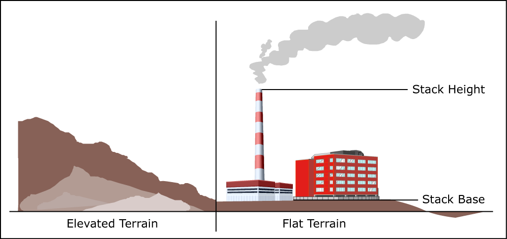
5.3.2 Flat and Complex Terrain
The models consider three different categories of terrain as follows:
- Complex Terrain: as illustrated in Figure 5.1, where terrain elevations for the surrounding area, are above the top of the stack being evaluated in the air modelling analysis.
Figure 5.1: Complex Terrain Conditions
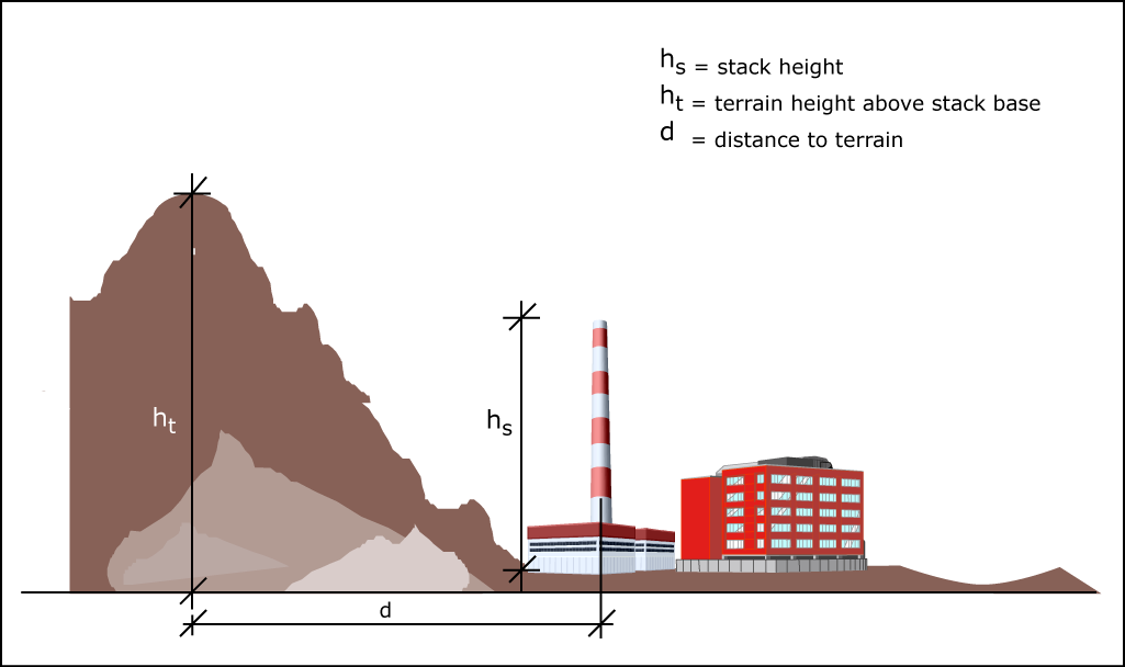
- Simple Terrain: where terrain elevations for the surrounding area are not above the top of the stack being evaluated in the air modelling analysis. The “Simple” terrain can be divided into two categories:
- Simple Flat Terrain is used where terrain elevations are assumed not to exceed stack base elevation. If this option is used, then terrain height is considered to be 0.0 m.
- Simple Elevated Terrain, as illustrated in Figure 5.2 is used where terrain elevations exceed stack base but are below stack height.
Figure 5.2: Simple Elevated and Flat Terrain Conditions
5.3.3 Criteria for Use of Terrain Data
Section 16 of the Regulation sets out when terrain must be used. Section 16 of the Regulation states:
Terrain data
“16. (1) If an approved dispersion model is used for the purposes of this Part with respect to any point of impingement that has an elevation higher than the lowest point from which the relevant contaminant is discharged from a source of contaminant, the model shall be used in a manner that employs terrain data.
(2) This section does not apply if the approved dispersion model that is used is,
- the ASHRAE method of calculation;
- the method of calculation required by the Appendix to Regulation 346; or
- a dispersion model or combination of dispersion models that, pursuant to subsection 7 (3), is deemed to be included in references in this Part to approved dispersion models, if the dispersion model or combination of dispersion models is not capable of using terrain data.”
Evaluation of terrain within a study area is the responsibility of the modeller. It should be kept in mind that both the terrain elevation relative to the source release heights and the proximity of the terrain features to the facility affect the impact of terrain on the modelled concentration of contaminants at point of impingements. Screening model runs (i.e., SCREEN3) could be used to determine if terrain features could result in higher concentrations.
5.3.4 Obtaining Terrain Data
Digital elevation model (DEM) data covering Ontario suitable for use with AERMOD is available at the ministry’s Map: Regional Meteorological and Terrain Data for Air Dispersion Modelling website. The DEM data is in 7.5 minute format data (resolution 1:25,000) which can be used directly with the AERMOD terrain pre-processor AERMAP.
Terrain data is also available from Natural Resources Canada. It is in a format called CDED (Canadian Digital Elevation Data), and can be obtained at 1-degree or 15-minute spatial resolutions. The ministry prefers the use of the data available on the ministry website.
5.3.5 Preparing Terrain Data for Model Use
AERMAP is the digital terrain pre-processor for the AERMOD model. It analyzes and prepares digital terrain data for use within an air dispersion modelling project. Early versions of AERMAP required that the digital terrain data files be in native United States Geological Survey (USGS) 1-degree or 7.5-minute DEM format. The most recent version of AERMAP accepts additional data formats, including the 15-minute USGS DEM format.
The CDEM format is very similar to the USGS DEM format. The CDEM 1-degree or 15-minute data types can be used directly with AERMAP without the need for any conversions. However, 1-degree data does not contain optimal resolution for most air dispersion modelling analyses and thus should not be used given that the above mentioned better resolution DEM data is available. Refer to Chapter 5.2.2 UTM on the UTM coordinate system.
5.4 Land Use Characterization
Land use plays an important role in air dispersion modelling from meteorological data processing to defining modelling characteristics such as urban or rural conditions. Land use information is required by paragraph 10 of subsection 26 (1) of the Regulation.
Contents of ESDM report (Section 26 of the Regulation)
“…10. A description of the local land use conditions, if meteorological data described in paragraph 2 of subsection 13 (1) was used when using an approved dispersion model for the purpose of this section…”
Land use data can be obtained from digital land-use maps. These maps will provide an indication into the dominant land use types within an area of study, such as industrial, agricultural, forested and others. This information can then be used to determine dominant dispersion conditions and estimate values for the critical surface characteristics which are surface roughness length, albedo, and the Bowen ratio.
In 2008 the US EPA released the AERSURFACE tool, part of the AERMOD modelling system, to assist users in the appropriate selection of surface characteristics in the vicinity of a facility or site. AERSURFACE was designed to use United States Geological Survey (USGS) National Land Cover Data 1992 (NLCD92), which includes 21 land cover categories. These characteristics are then input into AERMET which determines the appropriate dispersion parameters for each area/sector surrounding the site. Consult the AERSURFACE User’s Guide(31) for specific guidance on using AERSURFACE.
In cases where the necessary data is not available electronically, users should obtain land use data from appropriate municipal land use maps or from site-specific/area observations, and determine the surface characteristics manually, as described below in Chapters 5.4.1 – 5.4.3. Users should follow the recommendations for determining surface characteristics as presented in Chapter 3.1 Tier 1 Modelling of the AERMOD Implementation Guide, 2008(32) or Chapter 2.3 AERSURFACE Calculation Methods of the AERSURFACE User’s Guide. Note that the use of site-specific observations is always preferable to other data sources. The source data (maps) and resulting files should be submitted to EMRB for review prior to use.
It should also be noted that the seasonal characteristics in the AERSURFACE User’s Guides(31,32) are based on 5 categories rather than the traditional 4 seasons. However, this approach is more subjective, as it requires user decisions on the land use conditions during specific periods. As a result, the ministry has maintained use of the 4 traditional seasons, in a manner consistent with the seasonal definitions in AERMOD. These are as follows:
- winter (December – February)
- spring (March – May)
- summer (June – August)
- autumn (September – November)
These periods should be used to apply any seasonal variations in surface characteristics.
5.4.1 Surface Roughness Length [m]
The surface roughness length, also referred to as surface roughness height, is a measure of the height of obstacles to the wind flow. Surface roughness affects the height above local ground level that a particle moves from the ambient air flow above the ground into a “captured” deposition region near the ground. This height is not equal to the physical dimensions of the obstacles, but is generally proportional to them. For many modelling applications, the surface roughness length can be considered to be on the order of one tenth of the height of the roughness elements.
Figure 5.3: Effect of Surface Roughness
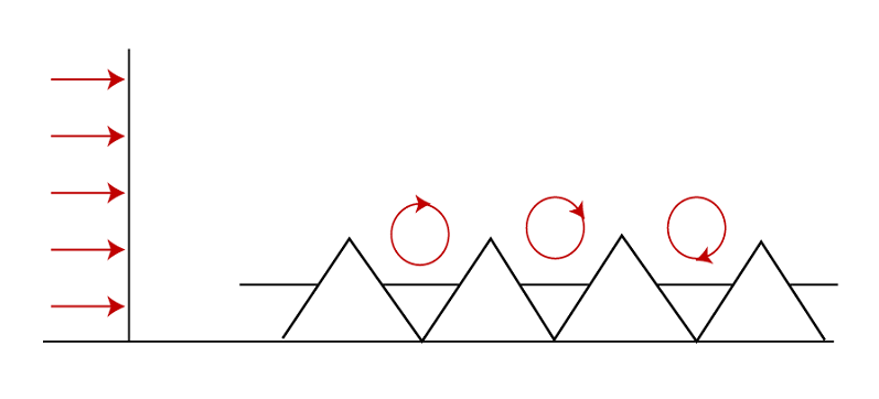
Table 5-1 lists typical surface roughness lengths for a range of land-use types as a function of season.
| Class Number | Land Use Class Name | Spring | Summer | Autumn | Winter |
|---|---|---|---|---|---|
| 11 | Open Water | 0.001 | 0.001 | 0.001 | 0.001 |
| 12 | Perennial Ice/Snow | 0.002 | 0.002 | 0.002 | 0.002 |
| 21 | Low Intensity Residential | 0.4 | 0.4 | 0.4 | 0.3 |
| 22 | High Intensity Residential | 1 | 1 | 1 | 1 |
| 23 | Commercial/Industrial/Transportation (Airport) | 0.07 | 0.07 | 0.07 | 0.07 |
| 23 | Commercial/Industrial/ Transportation (Other) | 0.7 | 0.7 | 0.7 | 0.7 |
| 31 | Bare Rock/Sand/Clay (AridRegion) | 0.05 | 0.05 | 0.05 | |
| 31 | Bare Rock/Sand/Clay (Non-aridRegion) | 0.05 | 0.05 | 0.05 | 0.05 |
| 32 | Quarries/Strip Mines/Gravel | 0.3 | 0.3 | 0.3 | 0.3 |
| 33 | Transitional | 0.2 | 0.2 | 0.2 | 0.2 |
| 41 | Deciduous forest | 1 | 1.3 | 1.3 | 0.5 |
| 42 | Coniferous forest | 1.3 | 1.3 | 1.3 | 1.3 |
| 43 | Mixed Forest | 1.15 | 1.3 | 1.3 | 0.9 |
| 51 | Shrubland (Arid Region) | 0.15 | 0.15 | 0.15 | |
| 51 | Shrubland (Non-arid Region) | 0.3 | 0.3 | 0.3 | 0.15 |
| 61 | Orchards/Vineyards/Other | 0.2 | 0.3 | 0.3 | 0.05 |
| 71 | Grasslands/Herbaceous | 0.05 | 0.1 | 0.1 | 0.005 |
| 81 | Pasture/Hay | 0.03 | 0.15 | 0.15 | 0.01 |
| 82 | Row Crops | 0.03 | 0.2 | 0.2 | 0.01 |
| 83 | Small Grains | 0.03 | 0.15 | 0.15 | 0.01 |
| 84 | Fallow | 0.02 | 0.05 | 0.05 | 0.01 |
| 85 | Urban/Recreational Grasses | 0.015 | 0.02 | 0.015 | 0.005 |
| 91 | Woody Wetlands | 0.5 | 0.5 | 0.5 | 0.3 |
| 92 | Emergent Herbaceous Wetlands | 0.2 | 02 | 0.2 | 0.1 |
AERMOD allows wind direction dependent surface characteristics to be used in the processing of the meteorological data. The US EPA recommends that the surface roughness in a given wind sector be calculated using the area-weighted average of the differing values for each land use within a specified distance of the site, based on an inverse square distance relationship. The US EPA AERSURFACE User’s Guide allows a radius of influence of 0.1 to 5 km to be used for surface roughness calculations, with a recommended distance of 1 km. A radius of influence longer than 1 km would be a reasonable choice for lower roughness lengths. The US EPA 2009 AERMOD Implementation Guide(32) recommends that the assessment be performed at the meteorological tower site. It should be noted that when incorporating local land use conditions into dispersion modelling assessments for the ministry, the conditions surrounding the facility should be specified, rather than the meteorological tower. Also, given the relatively large size of many facilities and the building heights at these locations the ministry will continue to recommend that a 3 km distance from the facility be used when specifying local land use conditions unless the facility is located in an urban environment. For more information on locating a meteorological tower, please refer to “Operations Manual for Air Quality Monitoring in Ontario”, as amended.
The selection of wind direction and seasonally dependent land use is described in Chapter 5.4.4 Wind Direction and Seasonably Dependent Land Use. Alternative methods of determining surface roughness lengths may be used, but modellers that undertake the meteorological processing themselves should consult with the ministry (EMRB) prior to data processing (Tier 3 Modelling).
5.4.2 Noon-Time Albedo
Noon-time albedo is the fraction of the incoming solar radiation that is reflected from the ground when the sun is directly overhead (see Figure 5.4). Table 5-2 lists typical albedo values as a function of several land use types and season.
Figure 5.4: Variations in Albedo Ratios Depending on Ground Cover
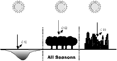
| Class Number | Land use Type | Spring | Summer | Autumn | Winter |
|---|---|---|---|---|---|
| 11 | Open Water | 0.1 | 0.1 | 0.1 | 0.1 |
| 12 | Perennial Ice/Snow | 0.6 | 0.6 | 0.6 | 0.7 |
| 21 | Low Intensity Residential | 0.16 | 0.16 | 0.16 | 0.45 |
| 22 | High Intensity Residential | 0.18 | 0.18 | 0.18 | 0.35 |
| 23 | Commercial/Industrial/Transportation (at Airport) | 0.18 | 0.18 | 0.18 | 0.35 |
| 23 | Commercial/Industrial/Transportation (Not at Airport) | 0.18 | 0.18 | 0.18 | 0.35 |
| 31 | Bare Rock/Sand/Clay (AridRegion) | 0.2 | 0.2 | 0.2 | |
| 31 | Bare Rock/Sand/Clay (Non-aridRegion) | 0.2 | 0.2 | 0.2 | 0.6 |
| 32 | Quarries/Strip Mines/Gravel | 0.2 | 0.2 | 0.2 | 0.6 |
| 33 | Transitional | 0.18 | 0.18 | 0.18 | 0.45 |
| 41 | Deciduous forest | 0.16 | 0.16 | 0.16 | 0.5 |
| 42 | Coniferous forest | 0.12 | 0.12 | 0.12 | 0.35 |
| 43 | Mixed Forest | 0.14 | 0.14 | 0.14 | 0.42 |
| 51 | Shrubland (Arid Region) | 0.25 | 0.25 | 0.25 | |
| 51 | Shrubland (Non-arid Region) | 0.18 | 0.18 | 0.18 | 0.5 |
| 61 | Orchards/Vineyards/Other | 0.14 | 0.18 | 0.18 | 0.5 |
| 71 | Grasslands/Herbaceous | 0.18 | 0.18 | 0.18 | 0.6 |
| 81 | Pasture/Hay | 0.14 | 0.2 | 0.2 | 0.6 |
| 82 | Row Crops | 0.14 | 0.2 | 0.2 | 0.6 |
| 83 | Small Grains | 0.14 | 0.2 | 0.2 | 0.6 |
| 84 | Fallow | 0.18 | 0.18 | 0.18 | 0.6 |
| 85 | Urban/Recreational Grasses | 0.15 | 0.15 | 0.15 | 0.6 |
| 91 | Woody Wetlands | 0.14 | 0.14 | 0.14 | 0.3 |
| 92 | Emergent Herbaceous Wetlands | 0.14 | 0.14 | 0.14 | 0.3 |
5.4.3 Bowen Ratio
The Bowen ratio is a measure of the amount of moisture at the surface. The presence of moisture at the earth’s surface alters the energy balance, which in turn alters the sensible heat flux and Monin-Obukhov length, which are both key dispersion parameters used by the AERMOD model. Table 5-3 lists Bowen ratio values as a function of land-use types, seasons and moisture conditions. Bowen ratio values vary depending on the surface wetness. Modellers shall use the average precipitation (moisture) conditions for selecting the Bowen ratio when processing meteorological data. If a modeller wishes to use other conditions, they should consult ministry (EMRB) prior to data processing (Tier 3).
| Class Number | Land Use Class Name | Spring | Summer | Autumn | Winter |
|---|---|---|---|---|---|
| 11 | Open Water | 0.1 | 0.1 | 0.1 | 0.1 |
| 12 | Perennial Ice/Snow | 0.5 | 0.5 | 0.5 | 0.5 |
| 21 | Low Intensity Residential | 0.8 | 0.8 | 1 | 0.5 |
| 22 | High Intensity Residential | 1.5 | 1.5 | 1.5 | 0.5 |
| 23 | Commercial/Industrial/Transportation (at Airport) | 1.5 | 1.5 | 1.5 | 0.5 |
| 23 | Commercial/Industrial/Transportation (Not at Airport) | 1.5 | 1.5 | 1.5 | 0.5 |
| 31 | Bare Rock/Sand/Clay (Arid Region) | 3 | 4 | 6 | |
| 31 | Bare Rock/Sand/Clay (Non-arid Region) | 1.5 | 1.5 | 1.5 | 0.5 |
| 32 | Quarries/Strip Mines/Gravel | 1.5 | 1.5 | 1.5 | 0.5 |
| 33 | Transitional | 1 | 1 | 1 | 0.5 |
| 41 | Deciduous forest | 0.7 | 0.3 | 1 | 0.5 |
| 42 | Coniferous forest | 0.7 | 0.3 | 0.8 | 0.5 |
| 43 | Mixed Forest | 0.7 | 0.3 | 0.9 | 0.5 |
| 51 | Shrubland (Arid Region) | 3 | 4 | 6 | |
| 51 | Shrubland (Non-arid Region) | 1 | 1 | 1.5 | 0.5 |
| 61 | Orchards/Vineyards/Other | 0.3 | 0.5 | 0.7 | 0.5 |
| 71 | Grasslands/Herbaceous | 0.4 | 0.8 | 1 | 0.5 |
| 81 | Pasture/Hay | 0.3 | 0.5 | 0.7 | 0.5 |
| 82 | Row Crops | 0.3 | 0.5 | 0.7 | 0.5 |
| 83 | Small Grains | 0.3 | 0.5 | 0.7 | 0.5 |
| 84 | Fallow | 0.3 | 0.5 | 0.7 | 0.5 |
| 85 | Urban/Recreational Grasses | 0.3 | 0.5 | 0.7 | 0.5 |
| 91 | Woody Wetlands | 0.2 | 0.2 | 0.3 | 0.5 |
| 92 | Emergent Herbaceous Wetlands | 0.1 | 0.1 | 0.1 | 0.5 |
| Class Number | Land Use Class Name | Spring | Summer | Autumn | Winter |
|---|---|---|---|---|---|
| 11 | Open Water | 0.1 | 0.1 | 0.1 | 0.1 |
| 12 | Perennial Ice/Snow | 0.5 | 0.5 | 0.5 | 0.5 |
| 21 | Low Intensity Residential | 0.6 | 0.6 | 0.6 | 0.5 |
| 22 | High Intensity Residential | 1 | 1 | 1 | 0.5 |
| 23 | Commercial/Industrial/Transportation (at Airport) | 1 | 1 | 1 | 0.5 |
| 23 | Commercial/Industrial/Transportation (Not at Airport) | 1 | 1 | 1 | 0.5 |
| 31 | Bare Rock/Sand/Clay (Arid Region) | 1 | 1.5 | 2 | |
| 31 | Bare Rock/Sand/Clay (Non-arid Region) | 1 | 1 | 1 | 0.5 |
| 32 | Quarries/Strip Mines/Gravel | 1 | 1 | 1 | 0.5 |
| 33 | Transitional | 0.7 | 0.7 | 0.7 | 0.5 |
| 41 | Deciduous forest | 0.3 | 0.2 | 0.4 | 0.5 |
| 42 | Coniferous forest | 0.3 | 0.2 | 0.3 | 0.5 |
| 43 | Mixed Forest | 0.3 | 0.2 | 0.35 | 0.5 |
| 51 | Shrubland (Arid Region) | 1 | 1.5 | 2 | |
| 51 | Shrubland (Non-arid Region) | 0.8 | 0.8 | 1 | 0.5 |
| 61 | Orchards/Vineyards/Other | 0.2 | 0.3 | 0.4 | 0.5 |
| 71 | Grasslands/Herbaceous | 0.3 | 0.4 | 0.5 | 0.5 |
| 81 | Pasture/Hay | 0.2 | 0.3 | 0.4 | 0.5 |
| 82 | Row Crops | 0.2 | 0.3 | 0.4 | 0.5 |
| 83 | Small Grains | 0.2 | 0.3 | 0.4 | 0.5 |
| 84 | Fallow | 0.2 | 0.3 | 0.4 | 0.5 |
| 85 | Urban/Recreational Grasses | 0.2 | 0.3 | 0.4 | 0.5 |
| 91 | Woody Wetlands | 0.1 | 0.1 | 0.1 | 0.5 |
| 92 | Emergent Herbaceous Wetlands | 0.1 | 0.1 | 0.1 | 0.5 |
| Class Number | Land Use Class Name | Spring | Summer | Autumn | Winter |
|---|---|---|---|---|---|
| 11 | Open Water | 0.1 | 0.1 | 0.1 | 0.1 |
| 12 | Perennial Ice/Snow | 0.5 | 0.5 | 0.5 | 0.5 |
| 21 | Low Intensity Residential | 2 | 2 | 2.5 | 0.5 |
| 22 | High Intensity Residential | 3 | 3 | 3 | 0.5 |
| 23 | Commercial/Industrial/Transportation (at Airport) | 3 | 3 | 3 | 0.5 |
| 23 | Commercial/Industrial/Transportation (Not at Airport) | 3 | 3 | 3 | 0.5 |
| 31 | Bare Rock/Sand/Clay (Arid Region) | 5 | 6 | 10 | |
| 31 | Bare Rock/Sand/Clay (Non-arid Region) | 3 | 3 | 3 | 0.5 |
| 32 | Quarries/Strip Mines/Gravel | 3 | 3 | 3 | 0.5 |
| 33 | Transitional | 2 | 2 | 2 | 0.5 |
| 41 | Deciduous forest | 1.5 | 0.6 | 2 | 0.5 |
| 42 | Coniferous forest | 1.5 | 0.6 | 1.5 | 0.5 |
| 43 | Mixed Forest | 1.5 | 0.6 | 1.75 | 0.5 |
| 51 | Shrubland (Arid Region) | 5 | 6 | 10 | |
| 51 | Shrubland (Non-arid Region) | 2.5 | 2.5 | 3 | 0.5 |
| 61 | Orchards/Vineyards/Other | 1 | 1.5 | 2 | 0.5 |
| 71 | Grasslands/Herbaceous | 1 | 2 | 2 | 0.5 |
| 81 | Pasture/Hay | 1 | 1.5 | 2 | 0.5 |
| 82 | Row Crops | 1 | 1.5 | 2 | 0.5 |
| 83 | Small Grains | 1 | 1.5 | 2 | 0.5 |
| 84 | Fallow | 1 | 1.5 | 2 | 0.5 |
| 85 | Urban/Recreational Grasses | 1 | 1.5 | 2 | 0.5 |
| 91 | Woody Wetlands | 0.2 | 0.2 | 0.2 | 0.5 |
| 92 | Emergent Herbaceous Wetlands | 0.2 | 0.2 | 0.2 | 0.5 |
5.4.4 Wind Direction and Seasonally Dependent Land Use
AERMET provides the ability to specify land use characteristics for up to 12 different contiguous, non-overlapping wind direction sectors that define unique upwind surface characteristics. Properties of wind sectors include:
- The sectors must be defined clockwise as the direction from which the wind is blowing, with north at 0°. (i.e. it is the upwind conditions that affect downwind dispersion)
- The sectors must cover the full circle so that the end value of one sector matches the beginning of the next sector.
- The beginning direction is considered part of the sector, while the ending direction is not.
Each wind sector can have a unique surface roughness length based on the weighted average of the land use categories within 3 km of the site for that sector. AERMET allows these surface characteristics to be specified annually, seasonally, or monthly to better reflect site conditions. For example, winter conditions can bring increased albedo values due to snow accumulation. Modellers should consult the AERSURFACE User’s Guide or contact EMRB for detailed guidance.
5.4.5 Defining Urban and Rural Conditions
SCREEN3:
SCREEN3: Requires a designation of the site as being in a predominantly urban or rural setting. The US EPA document Guideline on Air Quality Models (40 CFR Part 51, Appendix W(11) describes procedures for classifying sites as urban or rural, and requires that either a land use classification procedure or a population based procedure be used in this determination. The land use procedure is considered a more definitive criterion, and should be used by modellers for the purposes of the Regulation unless the ministry has indicated in writing that another procedure (e.g. the population density procedure) is acceptable.
Land Use Procedure: The land use within a 3 km radius around the facility sources is examined. If more than 50% of the area is accounted for by land use categories ranging from multi-family dwelling to commercial and industrial use it is classified as urban. Otherwise the site is classified as rural.
Population Density Procedure: Compute the average population density within a 3 km radius around the facility sources. The designation of urban or rural is the given by:
(a) If p > 750 people ⁄ km2, select the Urban option,
If p ≤ 750 people ⁄ km2, select the Rural option.
Note that the population density approach can lead to erroneous classification of urban and rural conditions, if applied incorrectly. For example, in highly industrialized areas, the population density may be low which would indicate a rural classification but the area is sufficiently built-up such that it would be more appropriately classified as urban using the land use approach. Modellers that want to use this approach should contact EMRB for additional guidance.
AERMOD:
The urban option in AERMOD is used to account for the urban heat island effect. Impacts of surface roughness, albedo and the Bowen ratio on turbulent mixing are taken into account in developing the meteorological data sets. In urban areas the direct input of heat and the trapping of long wave radiation between buildings can increase convective turbulence above the levels calculated in the AERMET pre-processor. Factors that affect the selection of the urban option in AERMOD include the population/urban intensity and the location of a facility relative to the urban core. If a facility is located close to the edge of an urban area, the urban heat island option would generally not be selected. Modellers are encouraged to contact ministry (EMRB) to discuss the selection of the urban option for more complex cases.
Footnotes
- footnote[14] Back to paragraph Note that the regulatory version of the AERMOD, AERMET, and ASHRAE models may not necessarily be the most recent version of these models. See Chapter 1.1 Applications of the Dispersion Models in the Regulation for more information on model versions.
- footnote[15] Back to paragraph Note: For the purposes of this ADMGO document, the terms “regulatory defaults” and “non-default” options refer to the US EPA nomenclature of defining various aspects of the dispersion models and do not necessarily refer to requirements within the Regulation.
- footnote[16] Back to paragraph Considering the modelling limitations and with a goal to reduce the complexity for modellers, the ministry is retaining the historical power exponent of n = 0.28 for conversion. A modeller or the ministry may, in special situations, demonstrate that the use of an alternative conversion approach may be more appropriate or required (see subsection 17(3) of the Regulation).
- footnote[17] Back to paragraph Note the ISCPRIME model was phased out of the Regulation on February 1, 2012.