References
10.0 References
- US EPA, 2004. User’s Guide for the AMS/EPA Regulatory Model – AERMOD. Office of Air Quality Planning and Standards, Research Triangle Park, NC, EPA-454/B-03-001.
- US EPA, 2014. Addendum - User’s Guide for the AMS/EPA Regulatory Model – AERMOD. Office of Air Quality Planning and Standards, Research Triangle Park, NC, EPA-454/B-03-001.
- Paine, R.J., R.W. Brode, R.B. Wilson, A.J. Cimorelli, S.G. Perry, J.C. Weil, A. Venkatram, W.D. Peters and R.F. Lee, 2003. AERMOD: The Latest Features and Evaluation Results. Paper # 69878 to be presented at the Air and Waste Management Association 96th Annual Conference and Exhibition, June 22-26, 2003. Air and Waste Management Association, Pittsburgh, PA 15222.
- Cimorelli, A.J., S.G. Perry, A. Venkatram, J.C. Weil, R.J. Paine, R.B. Wilson, R.F. Lee, W.D. Peters, R.W. Brode, J.O. Paumier, 2004: AERMOD: Description of Model Formulation. US EPA, EPA-454/R-03-004. Available from US EPA SCRAM website.
- US EPA, 1995. User’s Guide for the Industrial Source Complex (ISC3) Dispersion Models (Revised), Volume 1. EPA-454/B-95-003a. Office of Air Quality Planning and Standards, Research Triangle Park, NC.
- US EPA, 1995. User’s Guide for the Industrial Source Complex (ISC3) Dispersion Models, Volume II – Description of Algorithms. US EPA, Research Triangle Park, NC 27711. Available from US EPA SCRAM website as of January 2003.
- US EPA, 1997. Addendum to ISC3 User’s Guide – The Prime Plume Rise and Building Downwash Model. Submitted by Electric Power Research Institute. Prepared by Earth Tech, Inc., Concord, MA.
- US EPA, 2004. User’s Guide for the AERMOD Meteorological Pre-processor (AERMET). EPA-454/B-03-002. Office of Air Quality Planning and Standards, Research Triangle Park, NC.
- US EPA, 2004. User’s Guide for the AERMOD Terrain Pre-processor (AERMAP). EPA-454/B-03-003. Office of Air Quality Planning and Standards, Research Triangle Park, NC.
- US EPA, 2009. Addendum - User’s Guide for the AERMOD Terrain Pre-processor (AERMAP). EPA-454/B-03-003. Office of Air Quality Planning and Standards, Research Triangle Park, NC.
- US EPA, 2003. Appendix W to Part 51 Guideline on Air Quality Models, 40 CFR Part 51. US EPA, Research Triangle Park, NC. Available from US EPA SCRAM website.
- US EPA, 1992. Screening Procedures for Estimating the Air Quality Impact of Stationary Sources, Revised. EPA Publication No. EPA-454/R-92-019. US EPA, Research Triangle Park, NC.
- US EPA, 1995. SCREEN3 Model User’s Guide. EPA-454/B-95-004. Office of Air Quality Planning and Standards, Research Triangle Park, NC.
- ASHRAE, 2007. ASHRAE Handbook - HVAC Applications. American Society of Heating, Refrigerating and Air-Conditioning Engineers. (ISBN 1-931862-23-0).
- ASHRAE, 2011. ASHRAE Handbook - HVAC Applications. American Society of Heating, Refrigerating and Air-Conditioning Engineers. (ISBN 978-1936504077)
- US EPA, 1992. Workbook of Screening Techniques for Assessing Impacts of Toxic Air Contaminants (Revised). EPA-454/R-92-024. Office of Air Quality Planning and Standards, Research Triangle Park, NC.
- Beychok, M, 1979 Fundamentals of Stack Gas Dispersion, Irvine CA
- AERFlare spreadshet and User’s Guide – Alberta Environment Regulatory Flare Methodology (version 2.03).
- Briggs, G.A., 1974. Diffusion Estimation for Small Emissions. In ERL, ARL USAEC Report ATDL-106. US Atomic Energy Commission, Oak Ridge, TN.
- US EPA, 1993. Model Clearinghouse Memo 93-II-09. A part of the Model Clearinghouse Information Storage and Retrieval System (MCHISRS). Office of Air Quality Planning and Standards, US EPA, Research Triangle Park, NC 27711.
- Tikvart, J.A., 1993. “Proposal for Calculating Plume Rise for Stacks with Horizontal Releases or Rain Caps for Cookson Pigment, Newark, New Jersey,” a memorandum from J.A. Tikvart to Ken Eng, US EPA Region 2, dated July 9, 1993.
- US EPA, 2012. Memorandum on the Haul Road Workgroup Final Report Submission. Office of Air Quality Planning and Standards, US EPA, Research Triangle Park, NC 27711.
- US EPA, 1990. Stack Heights, Section 123, Clean Air Act, 40 CFR Part 51. US EPA, Research Triangle Park, NC.
- Schulman, L.L., D.G. Strimaitis and J.S. Scire, 2000: Development and evaluation of the PRIME plume rise and building downwash model. Journal of the Air & Waste Management Association, 50:378-390.
- US EPA, 1995. User’s Guide to the Building Profile Input Program, EPA-454/R-93-038, Office of Air Quality Planning and Standards, Research Triangle Park, NC.
- US EPA, 1985. Guideline for Determination of Good Engineering Practice Stack Height (Technical Support Document for the Stack Height Regulations) – Revised EPA-450/4-80-023R, US EPA, Research Triangle Park, NC.
- Tickvart, J. A., May 11, 1988. Stack-Structure Relationships, Memorandum to Richard L. Daye, US EPA.
- Tickvart, J. A., June 28, 1989. Clarification of Stack-Structure Relationships, Memorandum to Regional Modeling Contacts, Regions I-X, US EPA.
- Lee, R. F., July 1, 1993. Stack-Structure Relationships – Further clarification of our memoranda dated May 11, 1988 and June 28, 1989, Memorandum to Richard L. Daye, US EPA.
- Schulman, et al., 1997. Addendum - User’s Guide for the Industrial Source Complex (ISC3) Dispersion Models, Volume 1. Office of Air Quality Planning and Standards, Research Triangle Park, NC.
- US EPA, 2008. AERSURFACE User’s Guide, EPA-454/B-08-001, Office of Air Quality Planning and Standards, Research Triangle Park, NC.
- US EPA, 2009. AERMOD Implementation Guide, AERMOD Implementation Workgroup. Office of Air Quality Planning and Standards, Research Triangle Park, NC.
- Iqbal, M., 1983. An Introduction to Solar Radiation. Academic Press, New York, NY.
- Scire, J.S., D.G. Strimaitis, R.J. Yamartino, 2000. A User’s Guide for the CALPUFF Dispersion Model (Version 5). EarthTech Inc., Concord, Massachusetts.
- US EPA, 1995. User’s Guide for CAL3QHC Version 2: A Modeling Methodology for Predicting Contaminant Concentrations Near Roadway Intersections. EPA –454/R-92-006 (Revised). US EPA, Research Triangle Park, NC 27711.
- Eckhoff, P.A., and Braverman, T.N. 1995. Addendum to the User’s Guide to CAL3QHC Version 2. (CAL3QHCR User’s Guide) US EPA, Research Triangle Park, NC 27711.
- Caltrans, 1989. CALINE4 – A dispersion Model for Predicting Air Contaminant Concentrations Near Roadways, Final Report prepared by the Caltrans Division of New Technology and Research (Report No. FHWA/CA/TL-84/15).
- US EPA, 1988. User’s Guide to SDM - A Shoreline Dispersion Model EPA-450/4-88-017. US EPA, Research Triangle Park, NC 27711.
- US EPA, 2011. AERSCREEN User’s Guide EPA-454/B-11-001. US EPA, Research Triangle Park, NC 27711.
- US EPA, 1998. Interagency Workgroup on Air Quality Modeling (IWAQM) Phase 2 Summary Report and Recommendation for Modeling Long Range Transport Impacts. EPA-454/R-98-019. US EPA, Office of Air Quality Planning and Standards, Research Triangle Park, NC 27711.
Appendix A: Alternative Models
A-1. Acceptable Alternative Models
The following list contains alternative models that are currently accepted by the Ministry of Environment and Climate Change (ministry) for site-specific consideration.
- CALPUFF/CALMET
- CAL3QHCR
- SDM – Shoreline Dispersion Model
- Physical Modelling (i.e. wind tunnel assessments)
- AERSCREEN
Use of any alternative model (i.e. one that is not listed in subsection 6 (1) of the Regulation) requires approval from the Director, via issuance of a notice under subsection 7 (1) of the Regulation. Pre-consultation with EMRB and submission of a form to request the use of the specified model is required. The form for Request Under s.7(1) of Regulation 419/05 for Use of a Specified Dispersion Model is available online.
A-2. Alternative Model Use
A-2.1 Use of CALPUFF/CALMET
CALPUFF(34) is a puff model that is capable of fully accounting for hour-by-hour and spatial variations in wind and stability. Puff models, in general, perform well at downwind distances from a few kilometres to more than 100 km. CALPUFF contains additional algorithms that allow it to emulate AERMOD at short distances where puff models are generally less reliable. Further, CALPUFF has been evaluated and found to be reasonably accurate at distances up to 300 km. Thus, CALPUFF can be recommended for use for all distances up to 300 km.
CALPUFF is a more complex model with increased meteorological data requirements that is particularly useful in modelling situations that involve long-range transport (up to 300 km, light wind and calm conditions, wind reversals such as land–sea (or lake) breezes and mountain–valley breezes, and complex wind situations found in very rugged terrain). The meteorological data used by the CALPUFF system must be pre-processed by the CALMET meteorological model, and as such differs from the meteorology that is used for AERMOD. CALMET produces three dimensional wind fields that allow wind speeds and directions to vary, both in the horizontal and vertical directions. Therefore, the model inputs, run-time and data analysis aspects of using CALPUFF are much more time intensive than other models such as AERMOD.
The decision as to whether the use of CALPUFF is justified requires competent meteorological judgment. There are no hard and fast rules that can be applied. Situations where the use of CALPUFF could be justified include complex terrain, near large lakes and for facilities with very tall stacks.
A-2.2 Use of CAL3QHCR
CAL3QHCR(35,36) is a roadway dispersion model that can process a year of hourly meteorological data, with corresponding emissions, traffic and intersection signalization data. CAL3QHCR is particularly recommended for modelling of intersections. At signalized intersections, it accounts for idling emission rates from vehicles. CAL3QHCR calculates the concentrations in the vicinity of a roadway or intersection at averaging periods from 1-hour to annual. CAL3QHCR can accommodate up to 120 “links,” including both free-flowing roads and signalized intersections, and predict concentrations of carbon monoxide (CO), particulates (PM) and other inert contaminants within a few kilometres of the roadway. Its regulatory use in the US is for CO concentrations near roads and intersections.
A link may constitute a (nearly) straight section of road, a signalized intersection, a bridge, an elevated road on fill, or a cut (depressed) roadway. A curved road can be represented as a series of links. Traffic data can be either as a general function of hour-of-day and day-of-week, or every hour of the year, depending on the detail required. CAL3QHCR is particularly useful when the worst case meteorological conditions are not known in advance, requiring a year of meteorology to be run to identify a worst case. It is also useful for obtaining averaging periods longer than 1-hour (e.g., 8-hour, 24-hour, etc.) directly from the computations, without the need for conservative averaging period conversions.
CALINE4(37) is another roadway model designed to calculate a single 1-hour average concentration for a defined single hour of meteorological data for local roadways including intersections. This is most useful when a worst-case 1-hour meteorology (e.g. light wind parallel to the roadway) is known. If a worst case meteorology is not known, or direct calculation of longer averaging periods is required, the CAL3QHCR model would be a better choice.
A-2.3 Use of the Shoreline Dispersion Model
The SDM (Shoreline Dispersion Model(38)) can calculate a year or more of hourly concentrations including the effect of shoreline fumigation on plumes from stack sources located near a body of water. Shoreline fumigation is only included when conditions exist such that the event is likely to occur. At other times, it calculates concentrations based on a standard Gaussian plume model. SDM is relatively easy to use, and is appropriate for sources located at a shoreline. The data requirements and ease of use are typical of Gaussian plume models.
Use of SDM to assess the potential concentrations due to shoreline fumigation conditions would typically be done in combination with the AERMOD model to assess concentrations during non-fumigation conditions. More complicated situations may require the use of CALPUFF which requires more time and data as described above.
A-2.4 Use of Physical Modelling
Physical modelling is a term that comprises modelling in a wind tunnel or water channel. Some situations are sufficiently complex that the available computer models cannot be relied upon. In such cases, the use of physical modelling may be considered. Physical modelling is without question the most costly of any modelling approach. Further, it can account for only one meteorological event at a time. Often, only neutral and stable conditions can be modelled. Even with these limitations, physical modelling can provide useful information for complex situations that cannot be reliably simulated by computer models.
A-2.5 Use of AERSCREEN
AERSCREEN is a screening-level air quality model based on the AERMOD dispersion algorithms. AERSCREEN is currently the preferred screening model in the US EPA list of dispersion models. This model consists of two main components: 1) the MAKEMET program which generates a site-specific matrix of meteorological conditions for input to the AERMOD model; and 2) the AERSCREEN command-prompt interface program. The AERSCREEN interface makes use of the pre-processor programs AERMAP and BPIPPRM to automate the processing of terrain and building information respectively. Along with the meteorological file produced by MAKEMET, AERSCREEN interfaces with AERMOD using the SCREEN option on the CO MODELOPT card to perform the modelling runs. The SCREEN option in AERMOD restricts the averaging period to 1-hour averages while the AERSCREEN interface performs plume centreline calculations to find the receptor distance with the highest impact, similar to the automated distance option in SCREEN3.
The AERSCREEN User’s Guide(39) also lists a second method for running AERMOD in a screening mode. The stand-alone MAKEMET program can be used to generate the matrix of meteorological conditions and then AERMOD is run directly with the SCREEN option. The second approach allows more user flexibility in defining the receptor network, however the approach using the AERSCREEN interface should produce more conservative results depending on the receptor resolution selected when directly running of AERMOD with MAKEMET meteorological data. Note that applications running the AERSCREEN interface or directly running AERMOD with the SCREEN option are for single sources only. Results from multiple sources can be combined as discussed earlier in Chapter 3.1.2.
A-3. Explanation of Use Requirements
A-3.1 CALPUFF/CALMET
At a minimum, CALMET should be run using input data from three or more surface and upper air meteorological stations. In addition, output from a prognostic atmospheric model such as the Weather Research and Forecasting Model (WRF) or other similar meteorological models may be used to improve CALPUFF performance. CALPUFF can also be run in one of its screening modes, or with a single meteorological data source. This however, defeats the benefits of CALPUFF’s ability to account for spatial variations in the wind field. It still accounts for time variations in wind and stability, however, so there may, in some limited cases, be a benefit in running CALPUFF in this mode. It should, however, be run using CALMET developed meteorology, from several meteorological stations in the majority of cases.
Whenever possible, five years of meteorological data should be used to drive CALPUFF. However, if adequate data is sparse a shorter period of data may be used (subject to approval). Further, if there are breaks in the meteorological data, care should be taken that all months are adequately represented so that seasonal variations in meteorology are adequately accounted for.
CALPUFF also requires terrain and land use data.
CALPUFF has a large number of input options available, and as an alternative model the manner in which it is used must be acceptable to the Director. Modellers who wish to use CALPUFF should consult with the ministry regarding which model options will be used in the runs, prior to submitting modelling results using CALPUFF. It is preferable that this be done prior to issuance of the required Section 7 notice, as these conditions may be written into the notice. This will determine the current recommendations for the input options to be used, as well as the selection of meteorological data to be used. In general, the recommendations of the Interagency Workgroup on Air Quality Modelling (IWAQM) Phase 2 report(40), or any more recent recommendations, should be followed. The IWAQM recommendations notwithstanding, the MPDF option should be set to “1,” i.e., “yes,” so that CALPUFF will emulate AERMOD in the near field. The MPDF in CALPUFF selects the use of a probability density function (pdf) instead of a Gaussian function to describe the contaminant distribution through the plume in the vertical during convective (i.e., unstable) conditions for near-field calculations. This is the approach used in AERMOD.
Similar to the use of CALPUFF, applicants that intend to run the CALMET meteorological pre-processor themselves should have a written agreement with the ministry on the options to be set and the meteorological data to be used.
A-3.2 Line Source/ Roadway Dispersion Models
If roadway contributions to concentrations in a specific area are clearly secondary, emissions due to vehicle movements can typically be adequately included in AERMOD or CALPUFF modelling. In this case, roadway sources may be treated as volume or area/line sources in AERMOD or CALPUFF. If the impacts of individual roadways are more significant, a “roadway” or line source model should be considered. These include CALINE-4 or CAL3QHCR which can be used to assess the effects of the roadway alone. This would be appropriate if existing concentrations of a contaminant from other sources (e.g., CO) are either low or are well defined. If a “worst case” meteorology is defined (e.g., one metre per second wind speed parallel to the roadway, at F stability), then CALINE-4 can be used to predict the worst case 1-hour average concentration. This can be used as a screening estimate of maximum concentrations at longer averaging periods (e.g., 8-hour, 24-hour) by applying the averaging period conversion factors set out in section 17 of the Regulation.
More refined modelling for longer averaging periods should be completed using the CAL3QHCR model when the roadway emissions dominate the concentrations. CAL3QHCR(36) requires meteorological data pre-processed using MPRM, RAMMET or PCRAMMET. The model should be run for five years of meteorology, which is available from EMRB upon request.
A-3.3 Shoreline Models
In situations where water bodies affect the meteorology near the shoreline area significantly, CALPUFF would be the model of choice. However, CALPUFF requires substantial resources in terms of data, computer power and time. In the case where the dominant sources are located on a shoreline, and other sources in the area are clearly secondary, the SDM (Shoreline Dispersion Model(38)) may be used. SDM is a far simpler and less costly model to use than CALPUFF. It is a matter of professional judgement as to when shoreline effects are sufficient to warrant a shoreline model. For this reason, and for the reason that the model of choice may be more complicated to run (i.e. CALPUFF), it is important that the modeller pre-consult with EMRB before modelling using an alternative model is initiated.
Appendix B: Elimination of Meteorological Anomalies
An Example Case Study for the Elimination of Meteorological Anomalies From the Maximum Values Table for 1hr and 24hr Averaged Concentrations
In this Appendix, an example of the methodology for the elimination of meteorological anomalies is presented. Note that the elimination of these anomalies is optional. Model results will always be conservative if the meteorological anomalies are not eliminated.
Figure B.0.1 contains a sample AERMOD Output Pathway definition, and the four bolded lines were added to generate the MAXTABLE option. The MAXTABLE as specified below will give the top 100 modelled values across the entire modelling domain.
Figure B.0.1: Selecting the MAXTABLE Option in AERMOD
****************************************

**  AERMOD Output Pathway

****************************************

**

OU STARTING

	RECTABLE ALLAVE 1ST

	RECTABLE 1 1ST

	RECTABLE 24 1ST

	MAXTABLE ALLAVE 100

**  Auto-Generated Plotfiles

	PLOTFILE 1 ALL 1ST file.AP\01H1GALL.PLT

	PLOTFILE 24 ALL 1ST file.AP\24H1GALL.PLT

OU FINISHED
Once the model run is complete, a listing of the ranked concentrations can be retrieved from the model output file. Sample excerpts of an AERMOD output file are shown in Table B.0-1.and Table B.0-2, which contain a portion of the Maximum Value tables of ranked 1st to 80th for the 1-hr and 24-hr concentrations respectively. The following example illustrates the elimination of meteorological anomalies from the maximum values table for 1hr and 24hr averaged concentrations, and the identification of the final concentrations (or compliance points).
Step 1: Open the AERMOD output file using a text editor;
Step 2: Locate the 1-hr Maximum Values Table (“the maximum 100 1-hr average concentration values“), and print the number of pages containing the data (~4 pages). A sample excerpt is shown in Table B.1.
Step 3: The first column of the table shows the Rank (starting with 1); the second column shows the concentration; and the third column identifies the meteorological date and time of occurrence (first two digits designate the year). For each meteorological year, cross out the eight hours with the highest 1-hr concentrations starting from the beginning of the table. From Table B.1. the following hours can be eliminated:
- 1996 Rank: 3, 7, 9, 45, 47, 61, 68, 70 & 77
- 1997 Rank: 2, 6, 8, 22, 43, 46, 49, 56
- 1998 Rank: 5, 14, 19, 20, 23, 24, 28, 31
- 1999 Rank: 1, 4 & 5, 10, 11, 12, 16, 18, 26
- 2000 Rank: 13, 15, 17, 21, 25, 27, 29, 32
Note that the 4th and the 5th highest ranked concentrations occurred at different locations but in the same hour and thus both are eliminated. This also occurs for the 70th and 77th highest ranked concentrations.
Step 4: Once the total of forty 1-hr periods have been eliminated from the 5-year data set, the final concentration would be the remaining highest ranking concentration in the table – in this example, the final concentration is 62.98217 which is ranked 30th highest overall and occurs in 1999.
Step 5: Similarly, from the 24-hr Maximum Values Table (Table B.2.), cross out the highest 24-hr concentration for each meteorological year starting from the beginning of the table. From Table B.2., the following 24-hr periods can be eliminated: 1996 Rank 22; 1997 Rank 4; 1998 Rank 1 and Rank 18; 1999 Rank 9; 2000 Rank 6 as shown in the table below. For 1998, both Rank 1 and Rank 18 occur on the same day (at different locations) and thus both are eliminated since this is considered one meteorological anomaly.
Step 6: Once the total of five 24-hr periods have been eliminated, the final concentration for modelling would be the remaining highest ranking concentration in the table – in this example, the final concentration is 47.52893 which is ranked 2nd highest and occurs in 1998.
| Rank | Concentration | (YYMMDDHH) | at Receptor (XR,YR) of | Type |
|---|---|---|---|---|
| 1. | (99061006) | at (−100.00, 0.00) | DC | |
| 2. | 97120410 | at (100.00, 0.00) | DC | |
| 3. | (96012310) | at (0.00, −100.00) | DC | |
| 4. | (99071606) | at (100.00, 0.00) | DC | |
| 5. | (98071606) | at (100.00, 100.00) | DC | |
| 6. | (97082119) | at (100.00, 0.00) | DC | |
| 7. | (96062920) | at (0.00, 100.00) | DC | |
| 8. | (97081219) | at (−100.00, 0.00) | DC | |
| 9. | (96022809) | at (100.00, 0.00) | DC | |
| 10. | (99120716) | at (100.00, 0.00) | DC | |
| 11. | (99082419) | at (−100.00, 0.00) | DC | |
| 12. | (99082005) | at (0.00, −100.00) | DC | |
| 13. | (00021609) | at (100.00, 0.00) | DC | |
| 14. | (98041819) | at (100.00, 0.00) | DC | |
| 15. | (00101608) | at (−100.00, 0.00) | DC | |
| 16. | (99120416) | at (100.00, 0.00) | DC | |
| 17. | (00062102) | at (0.00, 100.00) | DC | |
| 18. | (99082621) | at (−100.00, 0.00) | DC | |
| 19. | (98050824) | at (0.00, −100.00) | DC | |
| 20. | (98110617) | at (100.00, 0.00) | DC | |
| 21. | (00061501) | at (0.00, 100.00) | DC | |
| 22. | (97021907) | at (0.00, 100.00) | DC | |
| 23. | (98061121) | at (−100.00, 0.00) | DC | |
| 24. | (98041419) | at (−100.00, 0.00) | DC | |
| 25. | (00061323) | at (−100.00, 0.00) | DC | |
| 26. | (99061005) | at (−100.00, 0.00) | DC | |
| 27. | (00050506) | at (100.00, 0.00) | DC | |
| 28. | (98062524) | at (−100.00, 0.00) | DC | |
| 29. | (00102423) | at (0.00, −100.00) | DC | |
| 30. | 62.98217 | (99101719) | at (0.00, −100.00) | DC |
| 31. | (98022718) | at (−100.00, 0.00) | DC | |
| 32. | (00030618) | at (0.00, 100.00) | DC | |
| 33. | 62.94170 | (98112009) | at (0.00, −100.00) | DC |
| 34. | 62.91700 | (00121621) | at (−100.00, 0.00) | DC |
| 35. | 62.91359 | (99121305) | at (0.00, −100.00) | DC |
| 36. | 62.91128 | (00031921) | at (−100.00, 0.00) | DC |
| 37. | 62.89389 | (98120509) | at (−100.00, 0.00) | DC |
| 38. | 62.86679 | (99081902) | at (0.00, −100.00) | DC |
| 39. | 62.83199 | (00022101) | at (100.00, 0.00) | DC |
| 40. | 62.82443 | (98111003) | at (−100.00, 0.00) | DC |
| 41. | 62.82240 | (00101302) | at (100.00, 0.00) | DC |
| 42. | 62.80699 | (00042122) | at (0.00, −100.00) | DC |
| 43. | (97012722) | at (0.00, 100.00) | DC | |
| 44. | 62.79989 | (99102108) | at (100.00, 0.00) | DC |
| 45. | (96091420) | at (0.00, 100.00) | DC | |
| 46. | (97012124) | at (0.00, 100.00) | DC | |
| 47. | (96120821) | at (100.00, 0.00) | DC | |
| 48. | 62.77896 | (99060906) | at (0.00, −100.00) | DC |
| 49. | (97121909) | at (100.00, 0.00) | DC | |
| 50. | 62.74012 | (00022608) | at (−100.00, 0.00) | DC |
| 51. | 62.72754 | (99031508) | at (0.00, −100.00) | DC |
| 52. | 62.72545 | (00122108) | at (0.00, 100.00) | DC |
| 53. | 62.71577 | (98111617) | at (−100.00, 0.00) | DC |
| 54. | 62.69680 | (98120517) | at (−100.00, 0.00) | DC |
| 55. | 62.69494 | (00031922) | at (−100.00, 0.00) | DC |
| 56. | (97020705) | at (100.00, 0.00) | DC | |
| 57. | 62.68309 | (99052302) | at (0.00, −100.00) | DC |
| 58. | 62.68141 | (00040721) | at (−100.00, 0.00) | DC |
| 59. | 62.67597 | (98012103) | at (0.00, −100.00) | DC |
| 60. | 62.65615 | (00022519) | at (−100.00, 0.00) | DC |
| 61. | (96060824) | at (−100.00, 0.00) | DC | |
| 62. | 62.65057 | (00121322) | at (−100.00, 0.00) | DC |
| 63. | 62.63590 | (00122401) | at (0.00, 100.00) | DC |
| 64. | 62.61233 | (99031001) | at (0.00, −100.00) | DC |
| 65. | 62.57222 | (00061504) | at (0.00, 100.00) | DC |
| 66. | 62.57042 | (98090203) | at (0.00, 100.00) | DC |
| 67. | 62.56813 | (00082419) | at (0.00, −100.00) | DC |
| 68. | (96091702) | at (0.00, −100.00) | DC | |
| 69. | 62.52769 | (97060203) | at (−100.00, 0.00) | DC |
| 70. | (96112822) | at (0.00, 100.00) | DC | |
| 71. | 62.51467 | (99092418) | at (0.00, −100.00) | DC |
| 72. | 62.48830 | (00013102) | at (100.00, 0.00) | DC |
| 73. | 62.48801 | (00092303) | at (−100.00, 0.00) | DC |
| 74. | 62.47909 | (00121104) | at (0.00, −100.00) | DC |
| 75. | 62.47895 | (00092301) | at (−100.00, 0.00) | DC |
| 76. | 62.47134 | (00090207) | at (0.00, −100.00) | DC |
| 77. | (96112822) | at (100.00, 0.00) | DC | |
| 78. | 62.43554 | (98122101) | at (−100.00, 0.00) | DC |
| 79. | 62.43499 | (96042105) | at (100.00, 0.00) | DC |
| 80. | 62.42564 | (99121509) | at (0.00, 100.00) | DC |
| Rank | Concentration | (YYMMDDHH) | at Receptor (XR,YR) of | Type |
|---|---|---|---|---|
| 1. | (98020424) | at (0.00, −100.00) | DC | |
| 2. | 47.52893 | (98020524) | at (0.00, −100.00) | DC |
| 3. | 43.21863 | (98012224) | at (−100.00, −50.00) | DC |
| 4. | (97031524) | at (100.00, 0.00) | DC | |
| 5. | 39.50042 | (98110224) | at (50.00, −100.00) | DC |
| 6. | (00041724) | at (−100.00, 0.00) | DC | |
| 7. | 39.21030 | (00042424) | at (0.00, −100.00) | DC |
| 8. | 39.20195 | (00071124) | at (0.00, −100.00) | DC |
| 9. | (99012224) | at (−100.00, 0.00) | DC | |
| 10. | 38.69060 | (98022524) | at (50.00, −50.00) | DC |
| 11. | 38.66324 | (99122324) | at (100.00, 0.00) | DC |
| 12. | 38.58439 | (97081824) | at (0.00, −100.00) | DC |
| 13. | 38.49494 | (99010524) | at (100.00, 50.00) | DC |
| 14. | 38.38240 | (98022424) | at (50.00, −100.00) | DC |
| 15. | 38.33889 | (99081824) | at (0.00, −100.00) | DC |
| 16. | 38.33855 | (97121024) | at (−100.00, −50.00) | DC |
| 17. | 38.30874 | (99032524) | at (0.00, −100.00) | DC |
| 18. | (99020424) | at (50.00, −100.00) | DC | |
| 19. | 38.17769 | (00120124) | at (0.00, −100.00) | DC |
| 20. | 38.17244 | (98101024) | at (50.00, −100.00) | DC |
| 21. | 38.16967 | (99121724) | at (100.00, 0.00) | DC |
| 22. | (96100924) | at (50.00, −100.00) | DC | |
| 23. | 37.95693 | (98100624) | at (−100.00, 0.00) | DC |
| 24. | 37.84420 | (98011624) | at (0.00, −100.00) | DC |
| 25. | 37.72802 | (96091824) | at (50.00, −100.00) | DC |
| 26. | 37.70357 | (98123124) | at (100.00, 50.00) | DC |
| 27. | 37.70138 | (99022124) | at (0.00, −100.00) | DC |
| 28. | 37.68097 | (98040524) | at (50.00, −100.00) | DC |
| 29. | 37.40958 | (00102824) | at (0.00, −100.00) | DC |
| 30. | 37.38273m | (99102524) | at (50.00, 50.00) | DC |
| 31. | 37.35784 | (97020624) | at (100.00, 0.00) | DC |
| 32. | 37.30082m | (99010424) | at (100.00, 50.00) | DC |
| 33. | 37.23205 | (96101024) | at (50.00, −100.00) | DC |
| 34. | 37.04751 | (00110524) | at (0.00, −100.00) | DC |
| 35. | 36.90880 | (99031324) | at (50.00, −100.00) | DC |
| 36. | 36.87509 | (97041924) | at (50.00, −100.00) | DC |
| 37. | 36.84701 | (99121424) | at (−100.00, 0.00) | DC |
| 38. | 36.71939 | (99022024) | at (0.00, −100.00) | DC |
| 39. | 36.71157 | (98090824) | at (50.00, −100.00) | DC |
| 40. | 36.68082 | (99091624) | at (0.00, −100.00) | DC |
| 41. | 36.57086 | (00050224) | at (0.00, −100.00) | DC |
| 42. | 36.31826 | (98103124) | at (50.00, −100.00) | DC |
| 43. | 36.28111 | (97011424) | at (50.00, 50.00) | DC |
| 44. | 36.19683 | (99010424) | at (50.00, 50.00) | DC |
| 45. | 36.11743 | (98032124) | (−50.00, −50.00) | DC |
| 46. | 36.02768 | (99092124) | at (0.00, −100.00) | DC |
| 47. | 35.96717 | (98021324) | at (0.00, −100.00) | DC |
| 48. | 35.92574 | (98020624) | at (50.00, −100.00) | DC |
| 49. | 35.58223 | (99011424) | (−50.00, −100.00) | DC |
| 50. | 35.57988 | (96121924) | at (100.00, 0.00) | DC |
| 51. | 35.50787 | (97021024) | at (100.00, 0.00) | DC |
| 52. | 35.47686 | (96110824) | at (50.00, −100.00) | DC |
| 53. | 35.47508 | (96040524) | at (50.00, −100.00) | DC |
| 54. | 35.36801 | (99112824) | at (100.00, 0.00) | DC |
| 55. | 35.32301 | (00122224) | at (100.00, 50.00) | DC |
| 56. | 35.25390 | (99042424) | at (0.00, −100.00) | DC |
| 57. | 35.24054 | (98122324) | at (100.00, 50.00) | DC |
| 58. | 35.20003 | (97091024) | at (−100.00, 50.00) | DC |
| 59. | 35.19956 | (96030624) | at (0.00, −100.00) | DC |
| 60. | 35.14633 | (97011124) | at (100.00, 50.00) | DC |
| 61. | 35.09946 | (96110124) | at (100.00, 50.00) | DC |
| 62. | 35.09356 | (99031324) | at (0.00, −100.00) | DC |
| 63. | 35.01658 | (00111824) | at (100.00, 0.00) | DC |
| 64. | 34.99058 | (96010224) | at (0.00, −100.00) | DC |
| 65. | 34.98722 | (97011324) | at (100.00, 50.00) | DC |
| 66. | 34.98309 | (98101124) | at (50.00, −100.00) | DC |
| 67. | 34.89045 | (00011724) | at (0.00, −100.00) | DC |
| 68. | 34.84517 | (97070424) | at (100.00, 0.00) | DC |
| 69. | 34.70854 | (98040624) | at (50.00, −100.00) | DC |
| 70. | 34.65571 | (98013024) | at (50.00, −50.00) | DC |
| 71. | 34.63356 | (98071024) | at (50.00, −100.00) | DC |
| 72. | 34.59713 | (98031024) | at (50.00, −50.00) | DC |
| 73. | 34.57745 | (98032724) | at (50.00, 50.00) | DC |
| 74. | 34.46351 | (99011324) | at (0.00, −100.00) | DC |
| 75. | 34.36126 | (99031924) | at (50.00, −50.00) | DC |
| 76. | 34.32848 | (98010324) | at (50.00, 50.00) | DC |
| 77. | 34.26509 | (97011124) | at (50.00, 50.00) | DC |
| 78. | 34.18020 | (98030824) | at (−100.00, 0.00) | DC |
| 79. | 34.09071 | (97110924) | at (50.00, −100.00) | DC |
| 80. | 34.06385 | (00122824) | at (0.00, −100.00) | DC |
Appendix C: Instructions on the Use of the Models in the “Appendix to Regulation 346”
C-1. Introduction and Applicability
Ontario Regulation 346 was the previous legislation under the Ontario Environmental Protection Act that regulated local air quality in the province of Ontario. The Appendix to Regulation 346 contained a mathematical description of three dispersion model calculations which were to be used to demonstrate compliance with ministry Two of those models, the Virtual Source model and the Point Source model have been translated into a software program known as the Regulation 346 Dispersion Modelling Package which is made available by the Ministry of the Environment.
O. Reg. 346 was replaced with Ontario Regulation 419/05 on November 30th, 2005. Subsection 6 (1) of the Regulation presents the list of approved dispersion models that, depending on a facility’s industrial classification (NAICS Code), must be used to demonstrate compliance with ministry POI Limits. “The method of calculation required by the Appendix to Regulation 346, if section 19 applies to the discharges..” is specified in paragraph 5 of subsection 6 (1), and thus is an approved dispersion model for applicable facilities, and can only be used to demonstrate compliance with Schedule 2 standards and guidelines (i.e. it can only be used if section 19 applies to discharges from the facility).
C-2. The Regulation 346 Dispersion Modelling Software
The Regulation 346 dispersion model is a simple, yet effective tool for calculating short-term (½ hour) maximum contaminant concentrations that result from contaminant emissions to air. The software package has been setup to search through the range of meteorological conditions specified in the regulation, at all ground level receptors located off the facility’s property to identify the meteorological condition which will give the highest half-hour average concentration at a point of impingement. In addition the Regulation 346 Package can calculate the concentration at specific points of impingement, such as air intakes on the roofs of nearby buildings or impingement on the sides or roof of an apartment building.
For most industrial operations, the POI at which the maximum half-hour concentration will occur is typically located on or beyond the facility property line. In some instances, emissions from adjacent properties or facilities are modelled together as a single facility with a single property boundary that includes all adjacent properties. The requirements for adjacent properties are outlined in section 4 of the Regulation. Where there is a potential for Same Structure Contamination, the concentration may need to be assessed inside the property line, using an additional approved dispersion model as detailed in subsection 9 (1) of the Regulation.
C-2.1. Model Sources
For the typical circumstance where the POI is located at or beyond a company’s property-line, the sources will be modelled as either virtual sources or point sources. The difference between whether a source can be considered a point or virtual source is determined by whether or not the release of the pollutant is mixed into the region beside a building due to the strong turbulent air currents near the building.
The key concept in deciding between a point and virtual source is the maximum building height. For the situation where the facility is a large rectangular structure the maximum building height will be the height of the highest point on that building excluding stacks, masts or small structures such as elevator penthouses. The following rules distinguish a point from a virtual source:
- A source can be considered a point source if the stack height above ground is more than twice the maximum building height (for buildings less than 20 metres high) otherwise the source is a virtual source;
- For a building greater than 20 metres high, the source is treated as a point source if the stack height is more than 20 metres above the roof height otherwise the source is a virtual source;
- An additional criterion occurs when a nearby tall building is upwind of the emission source. If a building higher than the height of the stack above the ground is within 100 m of the stack then when the wind blows from the tall building toward the emission source, the source is treated as a virtual source due to the tall building.
- Fugitive emissions from open sources from which the emissions are mixed into a volume of air prior to dispersing are typically modelled as virtual sources. Examples include roadways and material handling sources such as stockpile formation and vehicle loading.
C-2.1.1. Modelling with Virtual Sources
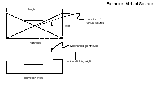
For a virtual source associated with a building, the emissions are assumed to be mixed into the turbulent region beside the building. An initial horizontal and vertical mixing which depends on the height and the width of the building is then used in the calculations. For virtual sources, the maximum concentration will occur along the property line. The parameters used in a virtual source calculation are: the contaminant emission rate, the maximum width, length and height (usually the maximum building height) of the virtual source, the location of the geometric centre of the virtual source, the orientation angle of the virtual source and the location of the property line.
The terms length and width have very specific meanings in the Appendix to Regulation 346. The building width is the shorter dimension. The building length is the longer dimension. The orientation is the acute angle formed by the building length intersecting the X-axis (default of 0 degrees). A counter-clockwise rotation increases the orientation. The location of the virtual source is the centre of the building (or source) when observed in the plan view.
For situations where the plant is a series of different buildings or sources the dispersion calculation can encompass all of them as one virtual source provided they are all connected or within 5 metres of each other. For these complicated virtual sources it is helpful to superimpose the rectangular shape of the virtual source on a copy of the plan view of the facility. The dimensions of the virtual source will be those of the smallest rectangle that can be constructed to encompass the contiguous structure. The maximum building (or source) height will be the height of the highest point on any of the structures that make up a significant portion of the overall virtual source excluding stacks, masts or small structures like elevator penthouses; and the location of the virtual source is the centre of the single rectangular building (or source) when observed in the plan view. Figure C.1.1 is an example of a virtual source that encompasses a number of individual buildings or tiers.
Figure C.2.1: Example Virtual Source
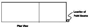
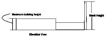
C-2.1.2. Modelling with Point Sources
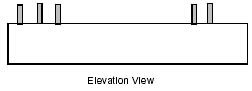
If the discharge takes place outside of the turbulent air currents near the building the emission would travel downwind as an elevated plume and then mix down to ground level some distance away. This elevated plume emission is known as a point source. For point sources the emissions released from the stack top will travel downwind as an elevated plume. The material would be slowly mixed horizontally and vertically. At some distance from the stack, the material would be mixed down to ground level resulting in the ground-level concentration maximum occurring a distance from the stack. Because emissions from a point source would have to be mixed horizontally and vertically over a significant volume before the plume is mixed to ground level, a given emission rate usually results in a smaller maximum ground-level concentration if it is released from a point source as opposed to a virtual source. The maximum concentration typically occurs at some distance away from the source usually also some distance away from the property-line. The important parameters used in a point source are: the contaminant emission rate, the discharge velocity, the discharge temperature, the stack diameter, the stack height and the stack location, the location of the property line and the location of any off site receptors that the plume may impact on. The emission source is treated as a point source if the stack is higher than the criteria described above. Figure C.2-2 shows an example of a point source.
Figure C.2-2: Example Point Source
C-2.1.3. Single Dispersion Sources
In the common circumstance where all emissions from a facility are emitted as a single virtual source, there is a very useful shortcut that can be employed. Since for a virtual source the emissions discharged from a building are released into the turbulent zone around the building all the discharges can be lumped together and considered to be emitted from a common virtual source (Figure C.2-3).
Figure C.2-3: Example - Single Virtual Source Scenario
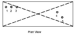
For this source configuration the emissions from Sources 1, 2, 3, 4 & 5 can be lumped together to be emitted from the one virtual source.
If these are the only sources then the dispersion calculation can be further simplified by running the virtual source once for a unit emission rate of 1 g/s. The resultant POI concentration at the property line can be used as a dispersion factor where the product of the dispersion factor and a contaminant emission rate is the POI concentration of that contaminant at the property line.
C-2.1.4. Complex Modelling Scenarios
While many industrial facilities can be described as a single virtual source there are other situations where a contaminant is emitted by more than one virtual or point source or a combination of many virtual and point sources. For these situations the modelling exercise is more complicated.
When there is more than one distinct virtual or point source that is emitting the contaminant the dispersion modelling exercise must be carried out for all the sources together and repeated for each individual contaminant.
C-3. Same Structure Contamination if Section 19 of O. Reg. 419 Applies
For most industrial operations, compliance with the point of impingement at which the maximum half-hour concentration will occur will be on or beyond the property line. There are, however some circumstances where the concentration needs to be assessed inside the property line (same structure contamination). This circumstance often occurs when the source is in an industrial mall, where the impact of contaminants released by tenants at one unit is assessed in terms of their impact on other neighbouring tenants in the building. The Regulation 346 model includes a very simplified calculation to estimate possible impacts of emission releases on air intakes, open doors or windows on the source’s own building. This approach can be used to assess same structure contamination if section 19 of the Regulation applies to discharges from a facility.
Regulation 346 addresses same structure contamination through use of the Scorer-Barrett equation. Concentrations depend on the stretched string distance from the release point of the emission source to the receptor (i.e., an air intake, a doorway or an operable window). The stretched string distance is the shortest distance from the release point to the receptor without intercepting the building.
Concentration (µg/m3) = 0.6 × 10⁶ × Emission Rate (g/s) ⁄ L2
Where,
- L
- 1.57 times the stretched string distance in metres (if the receptor is lower than the emission point);
otherwise,
- L
- the stretched string distance.
Note that the Scorer-Barrett equation may only be used by facilities for which section 19 applies. Facilities subject to section 20 of the Regulation (i.e. those required to use the US EPA models) are required to use the ASHRAE method for assessment of same structure contamination. ASHRAE may also be used to model same structure contaminant when section 19 applies.
C-4. Models in the Appendix to Regulation 346 Dispersion Modelling Package
Although there are ten programs included in the software package, only the first four programs are needed to assess compliance with Schedule 2 ministry POI Limits. Briefly, the purposes of those four programs in the Regulation 346 Dispersion Modelling Package are:
| Source Data Manager | Used to input information on the facility’s property line coordinates and on the emission source characteristics. |
|---|---|
| Point of Impingement Manager | Used to input information on the location of nearby buildings. |
| Maximum Ground Level Concentration | This program uses the files produced in the Source Data Manager and calculates the maximum half-hour Point of Impingement concentration outside of the facility’s property. |
| Concentrations at Points: | This program uses information from both data manager programs, (1) and (2), and calculates the maximum concentration at each receptor given in the Point of Impingement Manager. |
List of Routines:
- Source Data Manager
- Point of Impingement Data Manager
- Maximum Ground Level Concentration
- Concentration at Points
- Required Stack Height
- Isopleths
- Contour Printout
- Contour Plot
- General Concentration Plot
- Interpolation
Typical Inputs: Input default values are displayed within square brackets.
C-4.1. Description and Objective of the Various Programs and Routines
- Source Data Manager
Used to input the source and property line information in advance of running the concentration program. The output is stored in a file for later editing or use. This routine is essential if a property line is to be defined. It can also save a lot of typing time if multiple sources are to be run more than once.
- Point of Impingement Data Manager
Used to input the points of impingement in advance of running the concentration program. The output is stored in a file for later editing or use. This routine is not essential, but can save a lot of typing time if multiple receptors are to be run more than once.
- Maximum Ground Level Concentration
Used to compute the maximum ground level concentration from any combination of sources. If the property line has been defined, the program computes the maximum concentration off-property and on the property line. No point of impingement data is required.
- Concentration at Points
Used to compute the maximum concentration from any combination of sources at any combination of points of impingement. Both source and point of impingement data are required as input.
- Required Stack Height
Used to compute the height of stack required so that the maximum concentrations at ground level, at the property line and at points of impingement meet a specified standard. The program computes the height for only 1 source at a time.
- Isopleths
Used to compute concentration isopleths for any combination of point sources and Virtual Sources. The isopleths are computed over a grid superimposed over a vertical or horizontal plane. You may specify a particular stability, wind direction and wind speed. The result, stored in non-readable form, can be printed using Contour Printout or plotted using Contour Plot.
- Contour Printout
Used to print the results of an Isopleth or Interpolation run in readable form. Can be used to view contour results if a plotter is not available.
- Contour Plot
Used to plot the contours of a file created by Isopleth or Interpolation. The result can be routed to a plotter or to an output file (in non-readable form) for later plotting.
- General Concentration Plot
Used to compute and plot concentrations for any combination of sources. The concentrations are plotted along a line between two arbitrary endpoints. You may specify a particular stability, wind direction and wind speed. The result can be outputted to a plotter or to an output file (in non-readable form) for later plotting.
- Interpolation
Used to compute values over regularly spaced, points. The output is written to a file in non-readable form. The file can be subsequently outputted using Contour Printout or plotted using Contour Plot.
C-4.2. Model Input Parameters
Input parameters for the various routines are summarized below:
- Titling Information
e.g. Date, Title. All are optional. Be sure, though, to enter an output filename as the first input or else the program output will default to the printer.
- Point/Virtual Source
Indicates whether the source is a point source (e.g. a stack) or a virtual source (e.g. emission from a building vent).
- Emission Rate
In grams/second. For a single source, concentration (in µg/m3) is directly proportional to the emission rate.
- Stack Height
Enter the height of the stack from ground level to the top of the stack.
- Stack Diameter
Enter the inner stack diameter.
- Stack Exit Gas Velocity
If unknown, can be computed from flow rate and stack diameter.
- Coordinates
A local coordinate system is typically defined for the site. For example, this can be done by arbitrarily defining (0,0) at, the location of the largest source, or alternatively (0,0) could be defined as the location of the lower left corner of the property. All other coordinates are in metres, with the X-axis often chosen to represent the east-west direction.
- Building Width/Length/Orientation
The building width is the shorter dimension. The building length is the longer dimension. The orientation is the acute angle formed by the building length intersecting the X-axis (default of 0 degrees). A counter-clockwise rotation increases the orientation.
- Open/Closed Receptor
Used when entering an elevated (i.e. above ground level) receptor. A closed receptor will only allow concentration to be computed at the height specified. An open receptor will allow a search from ground level to the height specified for the maximum concentration at that (x,y) location.
- Selecting the Appropriate Building Height
Since many building have varying heights, it is important to select the appropriate building height relative to the wind direction and influence of taller portions of the building (or sections of a building) within a specific are of influence. Based upon information within the US EPA's “User’s Guide for the Industrial Source Complex (ISC3) Dispersion Models – Volume II – Description of Model Algorithms, September 1995”, the area of influence as a result of the taller portion of the building will be defined by a function of the distance L (where L is the lesser of the building height or the projected building width)…
- a distance of 5 times L from the edge of the taller portion for areas down-wind of the taller portion;
- a distance of 2 times L from the edge of the taller portion for areas up-wind of the taller portion; and
- a distance of 0.5 times L from the taller portion for areas parallel to the taller portion.
As discussed previously, for virtual sources the selected building height should be the height of the tallest building tier excluding stacks, masts or small structures such as elevator penthouses.
Summary of Commands for the Models in the Appendix to Regulation 346
The SDBMGR command options are as follows:
- RS - reset: prepares the program for a new data set;
- IN - input: input a source data set;
- ED - edit: edit a source data set; and
- LI - list: list a source data set.
SDBMGR edit command options are as follows:
- AS - add a source
- DS - delete a source
- MS - modify a source
- EH - edit the text header
- AP - add a point to the property-line
- DP - delete a point from the property-line
- MP - modify a point on the property-line